Supplement
G
Acceptance Sampling Plans
PROBLEMS
Operating Characteristic Curves
1. Alpha is the producer’s risk. To find Alpha, p is set equal to the acceptable quality
level (AQL = 0.5%). Then np = (200
0.005) = 1.00. From Table G.1 where c = 4,
( )
0.996P x c=
. Alpha
( )
1 0.996 0.004= − =
, or 0.4 percent.
Beta is the consumer’s risk. To find Beta, p is set equal to the lot tolerance proportion
defective. (LTPD = 4%). Then np = (200
0.04) = 8.0. From Table G.1 where c = 4,
( )
0.100P x c=
. Beta = 0.100, or 10 percent.
2. Hospital Supply.
a. p = 0.0010, n = 350.
np = (350)(0.0010) = 0.35.
b. np = (350)(0.0017) = 0.60.
c. If Alpha is required to be less than 5 percent,
( )
0.95 100% 5%
a
P−
. Given
a
3. Electronic components.
np = 1500(20/5000) = 6.0.
⚫
SUPPLEMENT G Acceptance Sampling Plans
G-2
Selecting a Single-Sampling Plan
4. Airline Maintenance
a. A variety of sampling plans will satisfy the requirements.
One such plan is n = 280, c = 6.
To find Alpha:
Acceptance Sampling Plans
⚫
SUPPLEMENT G
⚫
G-3
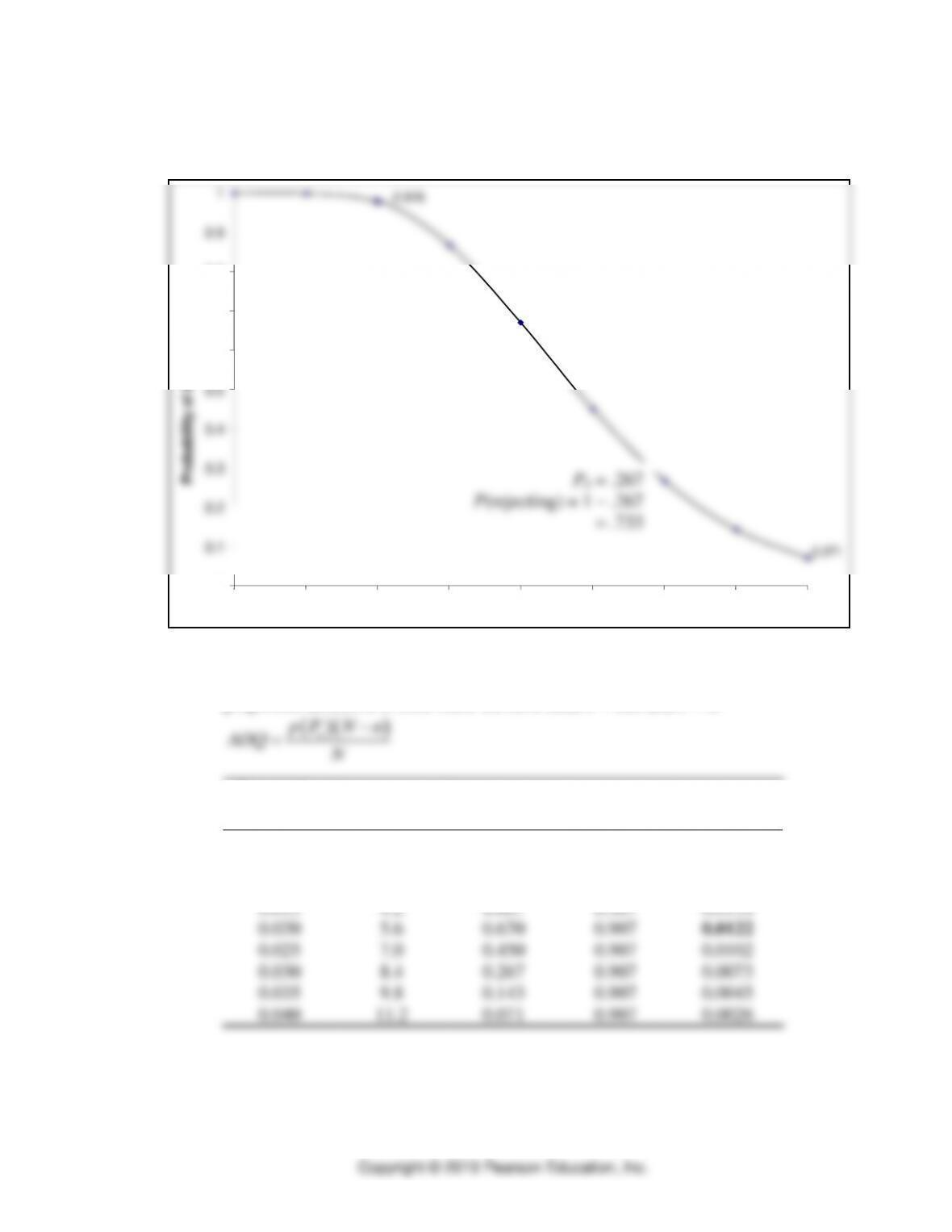
b. The OC curve is:
0.9
0.1
0.2
0.3
0.4
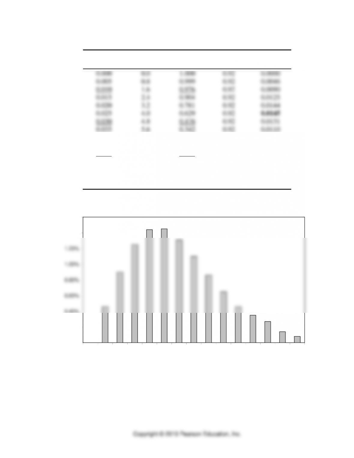
c. The maximum value of the AOQ over various possible values of the proportion
defective is 0.0122. The AOQL is therefore 1.22 percent defective when the lot
proportion defective is 0.02. Here we have used n = 280 and c = 6.
( )( )
a
p P N n
−
Proportion
Defective (p)
np
a
P
(N – n/N)
AOQ
0.000
0.0
1.000
0.907
0.0000
0.005
1.4
0.999
0.907
0.0045
0.010
2.8
0.976
0.907
0.0089
0.015
4.2
0.867
0.907
0.0118
0.020
5.6
0.670
0.907
0.0122
0.025
7.0
0.450
0.907
0.0102
0.030
8.4
0.267
0.907
0.0073
0.035
9.8
0.143
0.907
0.0045
0.040
11.2
0.071
0.907
0.0026
0
0.5
0.6
0.7
0.8
0
0.005
0.01
0.015
0.02
0.025
0.03
0.035
0.04
⚫
SUPPLEMENT G Acceptance Sampling Plans
G-4
5. Sunshine Shampoo Company.
AQL = 5/500, or 1%; LTPD = 5%.
a. Again, a variety of sampling plans will satisfy the requirements. One plan is
n = 160, c = 4.
To find Alpha:
b. np = 160(0.03) = 4.80.
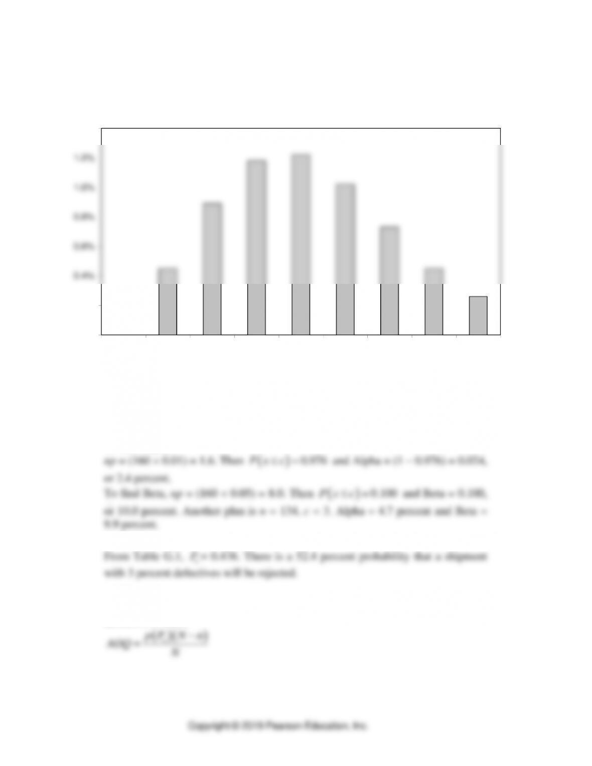
c. The maximum value of the AOQ over various possible values of the proportion
defective is 0.0145. The AOQL is 1.45 percent defective when the lot proportion
defective is 0.025.
( )( )
a
p P N n
−
Average Outgoing Quality, AOQ
0.0%
0.2%
0.4%
0.6%
0.8%
1.0%
1.2%
1.4%
0
0.005
0.01
0.015
0.02
0.025
0.03
0.035
0.04
Acceptance Sampling Plans
⚫
SUPPLEMENT G
⚫
G-5
Proportion
Defective (p)
np
a
P
(N – n/N)
AOQ
0.000
0.0
1.000
0.92
0.0000
0.005
0.8
0.999
0.92
0.0046
0.010
1.6
0.976
0.92
0.0090
0.015
2.4
0.904
0.92
0.0125
0.020
3.2
0.781
0.92
0.0144
0.025
4.0
0.629
0.92
0.0145
0.030
4.8
0.476
0.92
0.0131
0.035
5.6
0.342
0.92
0.0110
0.040
6.4
0.235
0.92
0.0086
0.045
7.2
0.156
0.92
0.0065
0.050
8.0
0.100
0.92
0.0046
0.055
8.8
0.070
0.92
0.0035
0.060
9.6
0.038
0.92
0.0021
0.065
10.4
0.023
0.92
0.0014
0.070
11.2
0.013
0.92
0.0008
AOQ x 100%
0.00%
0.20%
0.40%
0.60%
0.80%
1.00%
1.20%
1.40%
1.60%
0
0.005
0.01
0.015
0.02
0.025
0.03
0.035
0.04
0.045
0.05
0.055
0.06
0.065
0.07
⚫
SUPPLEMENT G Acceptance Sampling Plans
G-6
6. We can make a comparison by computing the producer’s and the consumer’s risk for
each plan using the Poisson Probabilities in Table G.1.
p = AQL = 1%
p = LTPD = 4%
Plan
np
a
P
np
a
P
1
n = 150, c = 4
1.5
0.981
1.9%
6.0
0.285
28.5%
2
n = 300, c = 8
3.0
0.996
0.4%
12.0
0.155
15.5%
The two plans are not equivalent. Increasing the sample size while maintaining the
same acceptance proportions (c/n) reduces risk to both parties.
7.
a.
n = 40, c = 1
p = AQL = 1%
p = LTPD = 5%
np
a
P
np
a
P
0.4
0.938
6.2%
2.0
0.406
40.6%
b. If we increase the acceptance number from 1 to 4 and increase the sample size to
160, we can improve the plan as follows:
n = 160, c = 4
p = AQL = 1%
p = LTPD = 5%
np
a
P
np
a
P
1.6
0.976
2.4%
8.0
0.100
10.0%
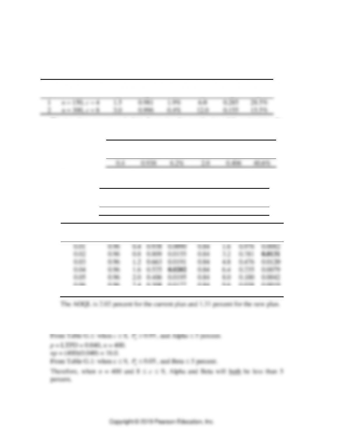
c.
Proportion
Current Plan n = 40, c = 1
New Plan n = 160, c = 4
Defective (p)
(N – n/N)
np
a
P
AOQ
(N – n/N)
np
a
P
AOQ
0.01
0.96
0.4
0.938
0.0090
0.84
1.6
0.976
0.0082
0.02
0.96
0.8
0.809
0.0155
0.84
3.2
0.781
0.0131
0.03
0.96
1.2
0.663
0.0191
0.84
4.8
0.476
0.0120
0.04
0.96
1.6
0.525
0.0202
0.84
6.4
0.235
0.0079
0.05
0.96
2.0
0.406
0.0195
0.84
8.0
0.100
0.0042
0.06
0.96
2.4
0.308
0.0177
0.84
9.6
0.038
0.0019
0.07
0.96
2.8
0.231
0.0155
0.84
11.2
0.013
0.0008
8. p = AQL = 0.010, n = 400.
np = (400)(0.010) = 4.0.
9. p = AQL = 0.010, c = 2.

Acceptance Sampling Plans
⚫
SUPPLEMENT G
⚫
G-7
In Table G.1, follow the c = 2 column down to 0.953 and read to the left to find
np = 0.80.
Since p = 0.01, n = 80.
10. In Table G.1, in the c = 10 column, the value 0.050 (or 0.049 approximately) is in the
row where np = 17.0.
11. A number of plans will satisfy the conditions for this problem. The most efficient
⚫
SUPPLEMENT G Acceptance Sampling Plans
G-8
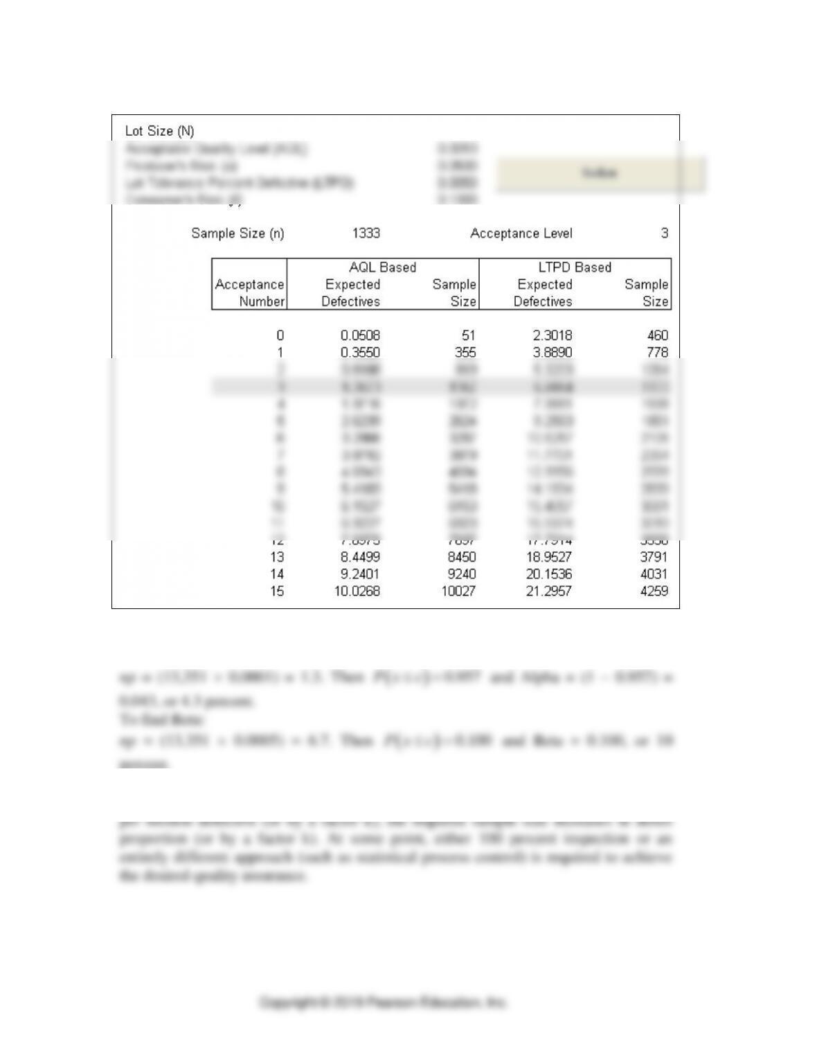
12. One plan is n = 13,351, c = 3.
To find Alpha:
percent.
It is observed that as the desired quality level increases from percent defective to parts
Acceptance Sampling Plans
⚫
SUPPLEMENT G
⚫
G-9
Average Outgoing Quality
13. a. AOQL = 0.00294, n = 509, c = 5.
b. i. When N is increased to 2000, AOQL = 0.0045, n = 509, c = 5.
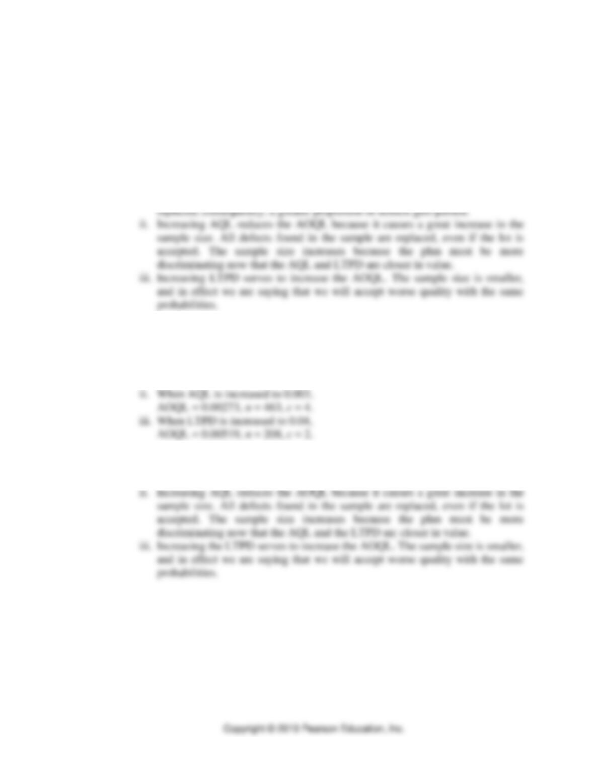
ii. When AQL is increased to 0.008, AOQL = 0.00042, n = 950, c = 12.
iii. When LTPD is increased to 0.06, AOQL =0.0121, n = 101, c = 2.
c. i. Increasing N raises the AOQL because the sample is a smaller proportion of
the total lot. When we accept the lot, only the defects in the sample are
14. Engine Plant
a. AOQL = 0.00264, n = 397, c = 3.
b. i. When N is increased to 2,000,
AOQL = 0.00351, n = 397, c = 3.
c. i. Increasing N raises the AOQL because the sample is a smaller proportion of
the total lot. When we accept the lot, only the defects in the sample are
replaced; consequently, a greater proportion of defects gets passed.