Supplement
E
Simulation
PROBLEMS
The Monte Carlo Simulation Process
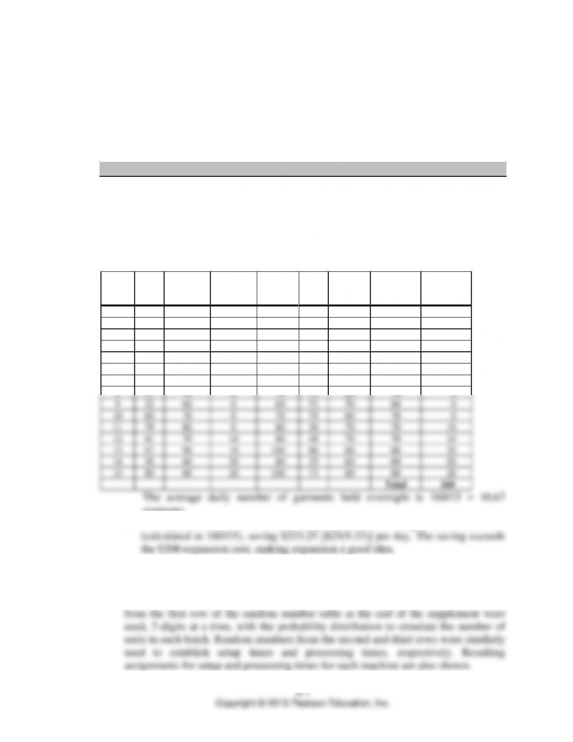
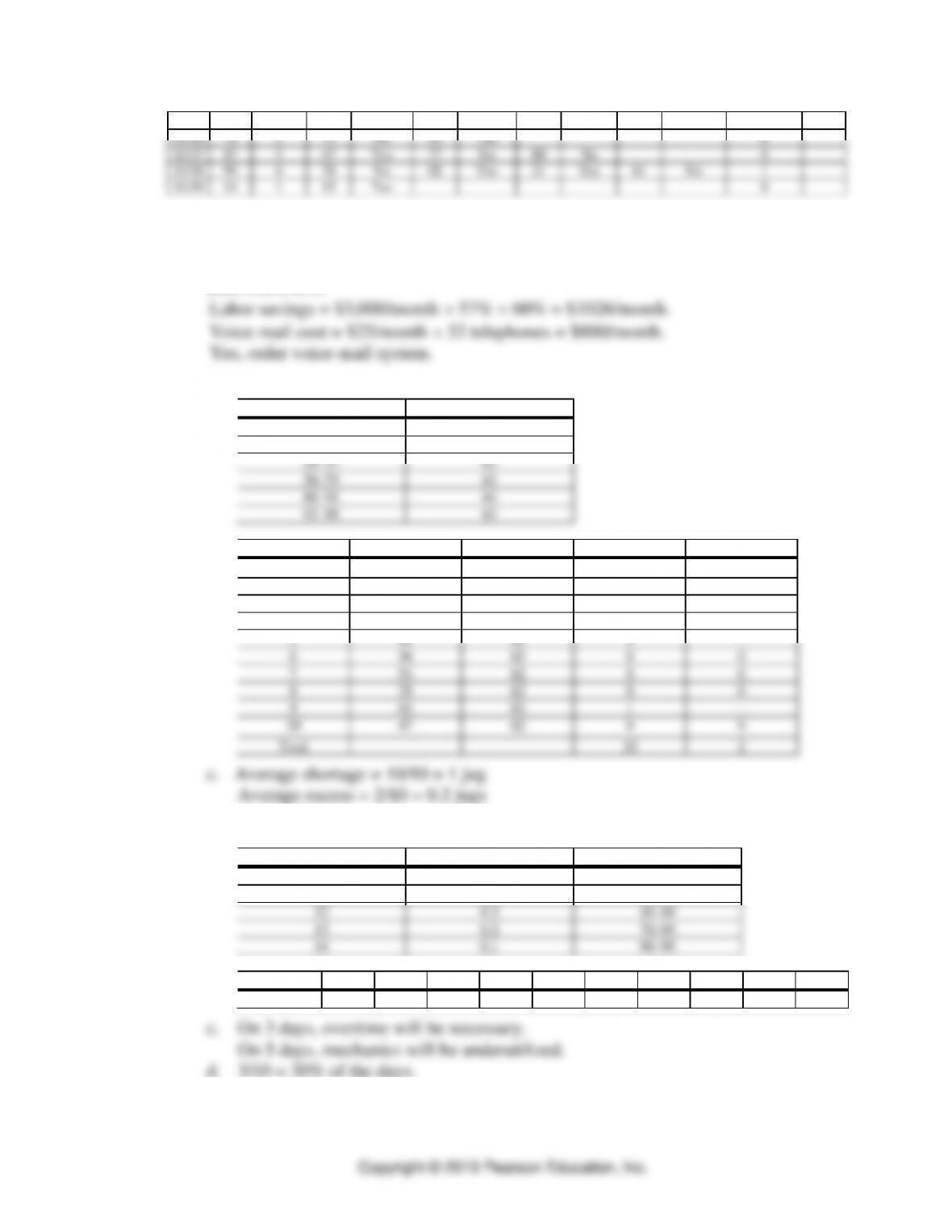
1. Comet Dry Cleaners
a. NGNC = Number of garments needing cleaning
MNGD = Maximum number of garments that could be dry cleaned
Day
RN
New
Garments
Queue at
Start
of Day
NGNC
RN
MNGD
Actual
Garments
Cleaned
Queue at
End
of Day
1
49
70
0
70
77
80
70
0
2
27
60
0
60
53
70
60
0
3
65
80
0
80
08
60
60
20
4
83
80
20
100
12
60
60
40
5
04
50
40
90
82
80
80
10
6
58
70
10
80
44
70
70
10
7
53
70
10
80
83
80
80
0
8
57
70
0
70
72
80
70
0
9
32
60
0
60
53
70
60
0
10
60
70
0
70
79
80
70
0
11
79
80
0
80
30
70
70
10
12
41
70
10
80
48
70
70
10
13
97
90
10
100
86
80
80
20
14
30
60
20
80
25
60
60
20
15
80
80
20
100
73
80
80
20
Total
160
The average daily number of garments held overnight is 160/15 = 10.67
garments.
b. The expansion reduces the number of garments held overnight from 20 to 10.67
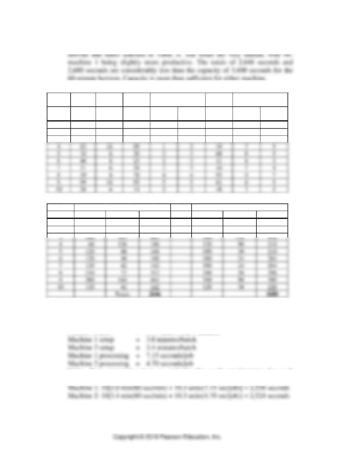
2. Precision Manufacturing Company.
The following Table A simulates the arrival of 10 batches over a 60-minute horizon.
With a different choice of random numbers, the results will vary. Random numbers
⚫
SUPPLEMENT E
⚫
Simulation
E-2
Table B determines the work requirements of each machine, based on the job
Table A Job arrivals, setup times, and processing times
Setup Times
(min)
Processing Times
(sec)
Batch
RN
Number
of Units
RN
Machine
1
Machine
2
RN
Machine
1
Machine
2
1
71
14
21
2
3
50
7
5
2
50
8
94
5
5
63
8
5
3
96
18
93
5
5
95
9
7
4
83
18
09
1
2
49
7
5
5
10
6
20
2
3
68
8
5
6
48
8
23
2
3
11
6
3
7
21
6
28
2
3
40
7
4
8
39
8
78
4
4
93
9
7
9
99
18
95
5
5
61
8
5
10
28
6
14
2
2
48
7
5
Table B Work Requirements
Machine 1 Requirements (sec)
Machine 2 Requirements (sec)
Batch
Setup
Processing
Total
Setup
Processing
Total
1
120
98
218
180
70
250
2
300
64
364
300
40
340
3
300
162
462
300
126
426
4
60
126
186
120
90
210
5
120
48
168
180
30
210
6
120
48
168
180
24
204
7
120
42
162
180
24
204
8
240
72
312
240
56
296
9
300
144
444
300
90
390
10
120
42
162
120
30
150
Totals
2646
2680
The small sample size of just 10 batches may cause us some estimation errors.
Another approach is to work with the expected values of the five probability
distributions. They can be computed as:
Number of jobs = 10.3 units every 6 minutes
Using these expected values to estimate the work requirements for each
machine for a 60-minute horizon, we get
Simulation
⚫
SUPPLEMENT E
⚫
E-3
3. Precision Manufacturing Company (II)
Because either machine has plenty of capacity, and continuing to assume equal
4. Omega University
a. Preliminary estimates or utilization and proportion of unanswered calls:
arrival rate: 90 calls per hour
60% forwarded to office = 54 calls/hour
only a few calls would go unanswered.
b. Simulation. See table showing the simulation.
The first three random numbers in the first row of the table are from the first
two digits in the second column of the Table of Random Numbers at the end of
c. Professors answered 34 calls (41%) and 48 (59%) were forwarded to the
department office. Of the 48 forwarded calls, only 34 calls (or 71%) were
⚫
SUPPLEMENT E
⚫
Simulation
E-4
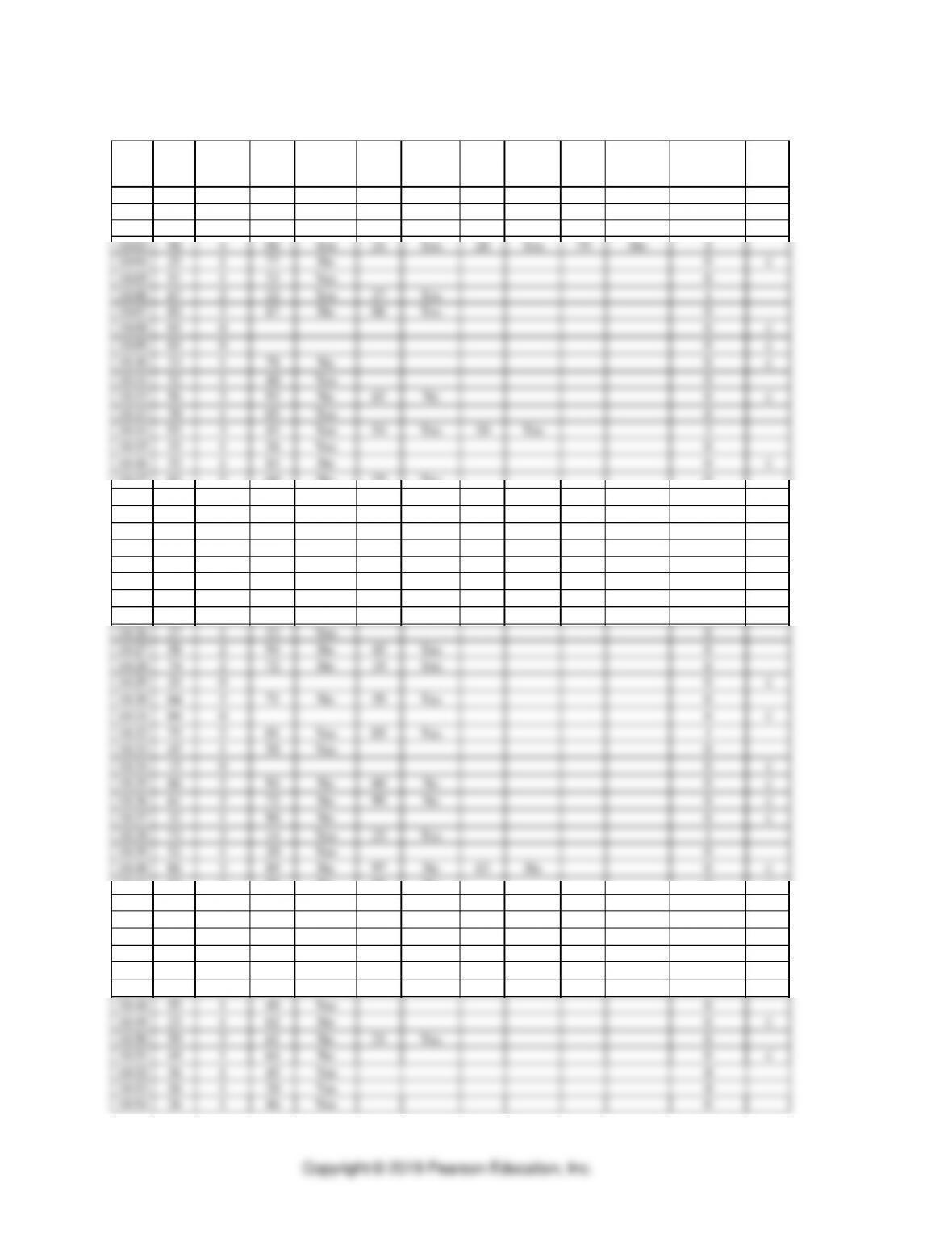
Table for Problem 4b: Simulation of Voice Mail System
Time
RN
No. of
Calls
Made
RN
1st Call
Forward?
(Yes/No)
RN
2nd Call
Forward?
(Yes/No)
RN
3rd Call
Forward?
(Yes/No)
RN
4th Call
Forward?
(Yes/No)
No. of
Calls Not
Answered
Asst
Idle
10:00
68
2
30
Yes
54
Yes
1
10:01
76
2
36
Yes
32
Yes
1
10:02
68
2
04
Yes
07
Yes
1
10:03
98
4
08
Yes
21
Yes
28
Yes
79
No
2
10:04
25
1
77
No
0
10:05
51
1
23
Yes
0
10:06
67
2
22
Yes
27
Yes
1
10:07
80
2
87
No
06
Yes
0
10:08
03
0
0
10:09
03
0
0
10:10
33
1
78
No
0
10:11
32
1
40
Yes
0
10:12
56
2
92
No
61
No
0
10:13
39
1
05
Yes
0
10:14
93
3
43
Yes
54
Yes
30
Yes
2
10:15
33
1
26
Yes
0
10:16
33
1
83
No
0
10:17
62
2
60
No
25
Yes
0
10:18
12
0
0
10:19
30
1
96
No
0
10:20
83
3
48
Yes
23
Yes
11
Yes
2
10:21
09
0
0
10:22
92
3
66
No
21
Yes
76
No
0
10:23
31
1
19
Yes
0
10:24
51
1
75
No
0
10:25
15
0
0
10:26
27
1
52
Yes
0
10:27
58
2
94
No
45
Yes
0
10:28
74
2
72
No
19
Yes
0
10:29
20
0
0
10:30
64
2
71
No
39
Yes
0
10:31
04
0
0
10:32
75
2
01
Yes
05
Yes
1
10:33
45
1
58
Yes
0
10:34
15
0
0
10:35
66
2
94
No
60
No
0
10:36
61
2
72
No
99
No
0
10:37
32
1
90
No
0
10:38
73
2
14
Yes
25
Yes
1
10:39
52
1
20
Yes
0
10:40
86
3
89
No
97
No
63
No
0
10:41
65
2
99
No
89
No
0
10:42
36
1
54
Yes
0
10:43
19
0
0
10:44
07
0
0
10:45
56
2
04
Yes
52
Yes
1
10:46
01
0
0
10:47
14
0
0
10:48
55
1
49
Yes
0
10:49
23
1
62
No
0
10:50
59
2
61
No
21
Yes
0
10:51
49
1
64
No
0
10:52
36
1
45
Yes
0
10:53
26
1
20
Yes
0
10:54
26
1
46
Yes
0
Simulation
⚫
SUPPLEMENT E
⚫
E-5
10:55
41
1
78
No
0
10:56
79
2
73
No
45
Yes
0
10:57
87
3
47
Yes
77
No
89
No
0
10:58
99
4
78
No
08
Yes
21
Yes
61
No
1
10:59
24
1
15
Yes
0
5. Omega University Voice mailboxes
The office assistant is currently spending 57% of his time answering the telephone.
See table showing the simulation. Assuming that time saved could be productively
used elsewhere,
6. E-Z Mart
a.
Random Number
Sales
00–09
60
10–23
61
24–57
62
58–79
63
80–91
64
92–99
65
b.
Trial
R.N.
Demand
Shortage
Excess
1
97
65
3
—
2
02
60
—
2
3
80
64
2
—
4
66
63
1
—
5
99
65
3
—
6
56
62
0
0
7
54
62
0
0
8
28
62
0
0
9
64
63
1
—
10
47
62
0
0
Total
10
2
c. Average shortage = 10/10 = 1 jug
Average excess = 2/10 = 0.2 jugs
7. Brakes-Only Service Shop
a.
# of Brake Jobs
Relative Frequency
Random Numbers
10
0.1
00–09
11
0.3
10–39
12
0.3
40–69
13
0.2
70–89
14
0.1
90–99
b.
RN
28
83
73
7
4
63
37
38
50
92
Demand
11
13
13
10
10
12
11
11
12
14
⚫
SUPPLEMENT E
⚫
Simulation
E-6
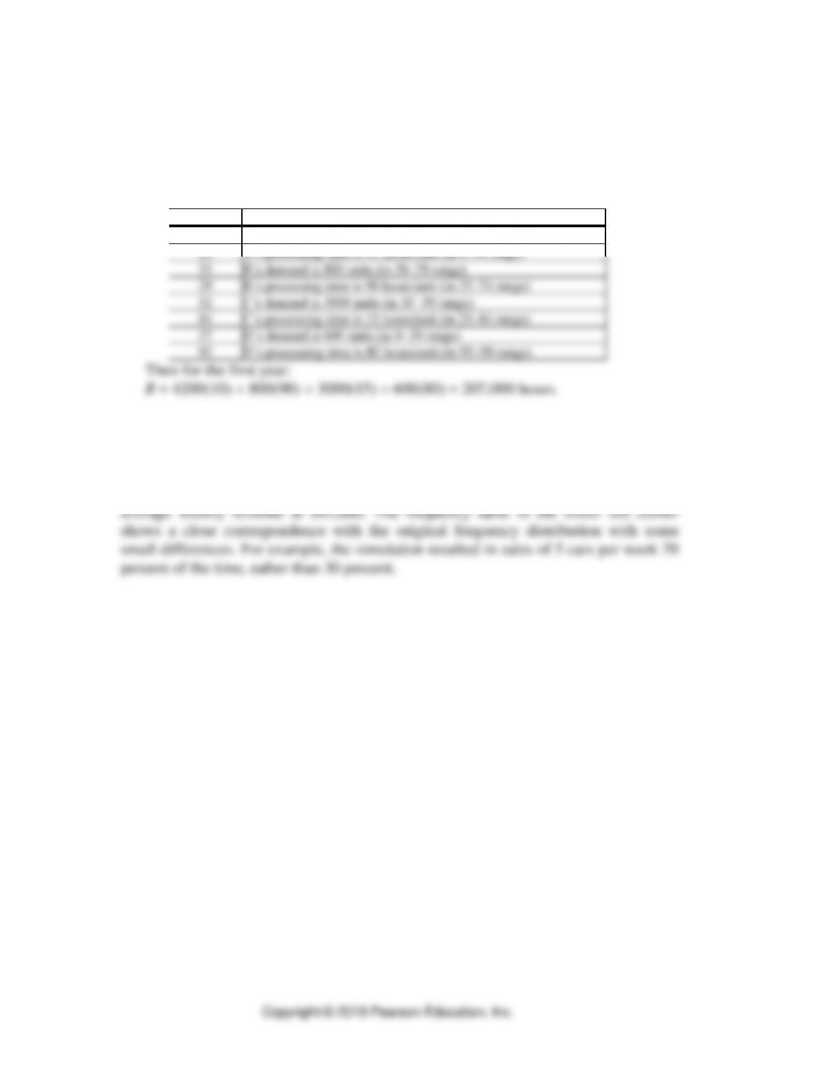
8. A machine center
a. Two random numbers could be used for each client—one for demand and one
for processing time. Once this has been done for all four clients, it is possible to
compute the value of R for the year just simulated. The result is one observation
for constructing a frequency chart or probability distribution.
b. For the first year simulated:
RN
Event
88
A’s demand is 4200 units (in 70–99 range)
24
A’s processing time is 10 hours/unit (in 0–34 range)
33
B’s demand is 800 units (in 30–79 range)
29
B’s processing time is 90 hours/unit (in 25–74 range)
52
C’s demand is 3000 units (in 10–59 range)
84
C’s processing time is 15 hours/unit (in 25–84 range)
37
D’s demand is 600 units (in 0–39 range)
92
D’s processing time is 80 hours/unit (in 95–99 range)
Then for the first year:
R = 4200(10) + 800(90) + 3000(15) + 600(80) = 207,000 hours.
Simulation with Excel Spreadsheets
9. BestCar sales activity
The spreadsheet follows, showing the average sales at 4.75 cars per week and the
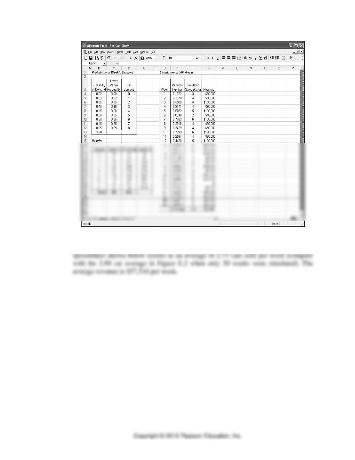
Simulation
⚫
SUPPLEMENT E
⚫
E-7
10. BestCar with price variability
Now there are two uncontrollable variables: weekly demand and sales price. The
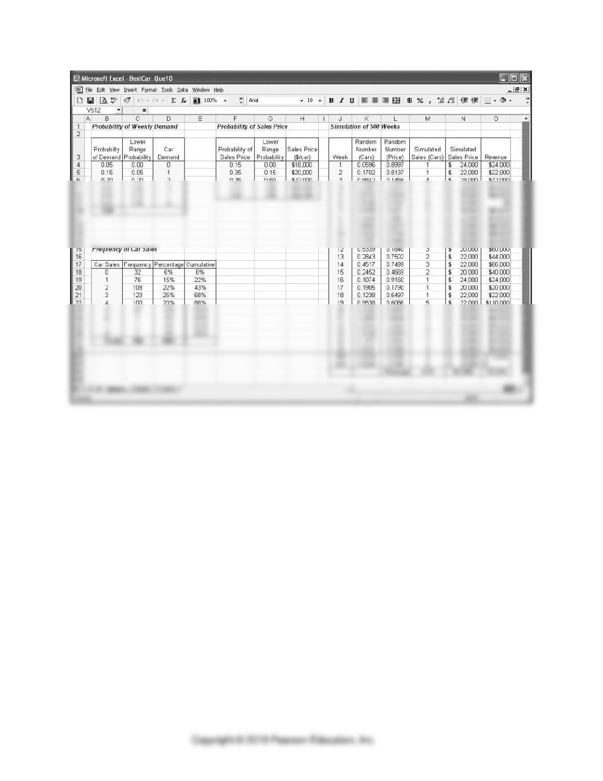
⚫
SUPPLEMENT E
⚫
Simulation
E-8