
Supplement
D Linear Programming
1. Characteristics of Linear Programming Models
1. Linear programming is an optimization process with several characteristics
a. Objective function:
b. Decision variables:
c. Constraints:
d. Feasible region:
e. Parameter or a coefficient:
• Certainty:
f. Linearity:
g. Nonnegativity:
2. Formulating a Linear Programming Model
1. Step 1: Define the decision variables.
a.
b.
2. Step 2: Write out the objective function
a.
b.
3. Step 3: Write out the constraints
a.
b.
c.
4. Application D.1: Problem Formulation for Crandon Manufacturing
The Crandon Manufacturing Company produces two principal product lines. One is a
portable circular saw, and the other is a precision table saw. Two basic operations are crucial
to the output of these saws: fabrication and assembly. The maximum fabrication capacity is
4000 hours per month; each circular saw requires 2 hours, and each table saw requires 1 hour.
The maximum assembly capacity is 5000 hours per month; each circular saw requires 1 hour,
and each table saw requires 2 hours. The marketing department estimates that the maximum
market demand next year is 3500 saws per month for both products. The average contribution
to profits and overhead is $900 for each circular saw and $600 for each table saw.
Management wants to determine the best product mix for the next year so as to maximize
contribution to profits and overhead. Also, it is interested in the payoff of expanding capacity
or increasing market share.
Definition of Decision Variables
1
x
=
2
x
=
Formulation
Maximize:
Subject to:
3. Graphic Analysis
1. What is the purpose of a graphic analysis?
2. Five basic steps (Examples D.2 and D.3)
a. Step 1: Plot the constraints
b. Step 2: Identify the feasible region
• Application D.2: Steps a and b for Crandon Manufacturing
Plot the constraints and shade the feasible region for Crandon Manufacturing, where:
2x1 + 1x2 ≤ 4,000 (Fabrication)
1x1 + 2x2 ≤ 5,000 (Assembly)
1x1 + 1x2 ≤ 3,500 (Demand)
x1, x2 ≥ 0 (Nonnegativity)
c. Step 3: Plot an objective function line (Example D.4)
• Corner points
• Iso-profit and iso-cost lines
d. Step 4: Find the visual solution
Constraint
Point 1
Point 2
x1
x2
x1
x2
1
( , )
( , )
2
( , )
( , )
3
( , )
( , )
• Application D.3 Steps c and d for Crandon Manufacturing
Plot one or more iso-profit lines line on graph on last page and picking the corner
point furthest from the origin. If not sue, draw addition lines parallel to first line until
optimal corner point is obvious. For our purposes:
Let Z = $2,000,000 (arbitrary choice)
Plot $900x1 + $600x2 = $2,000,000
Point 1
Point 2
Profit
x1
x2
x1
x2
$2,000,000
( , )
( , )
What corner point is furthest from the origin? What are its x1 and x2 values?
e. Step 5: Find the algebraic solution
• Step 1:
• Step 2:
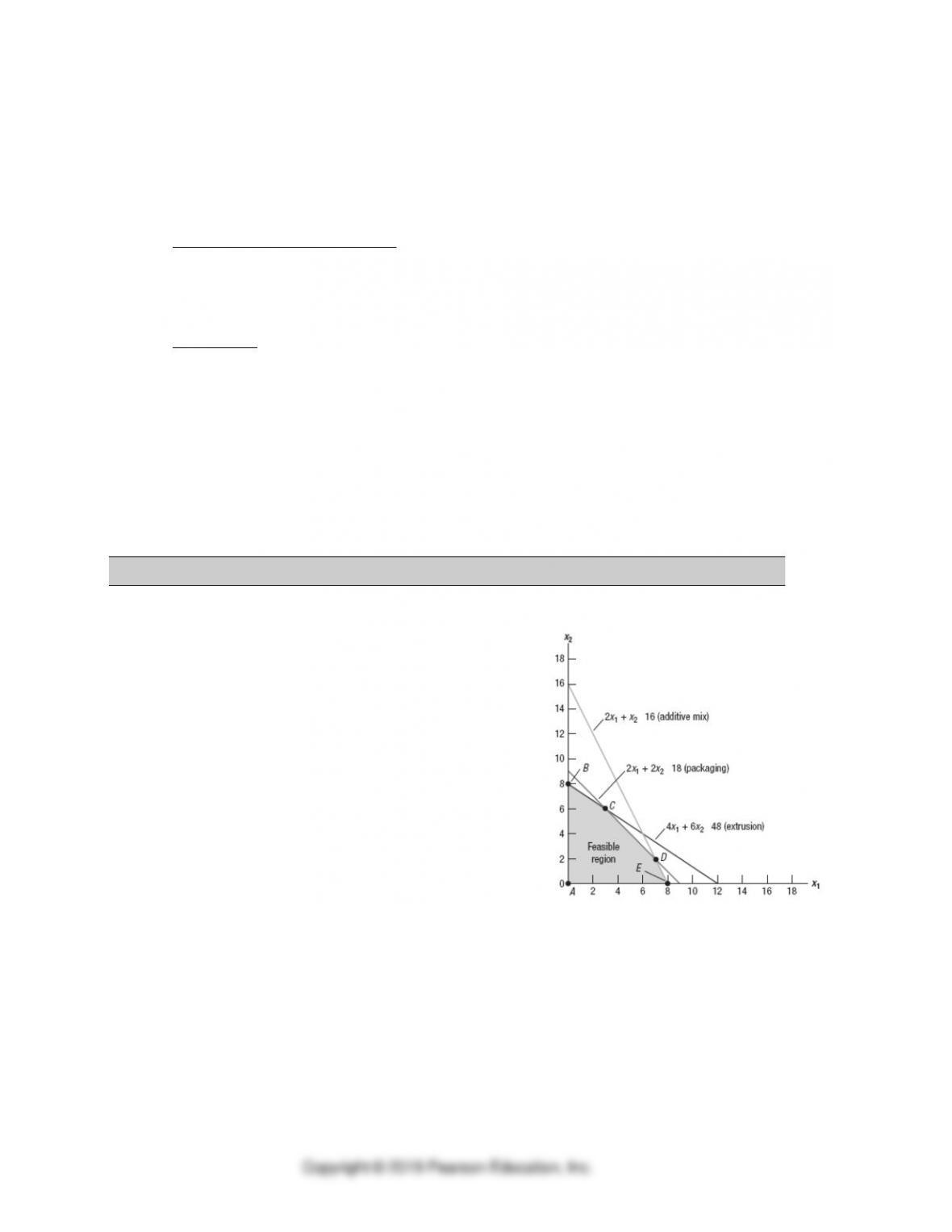
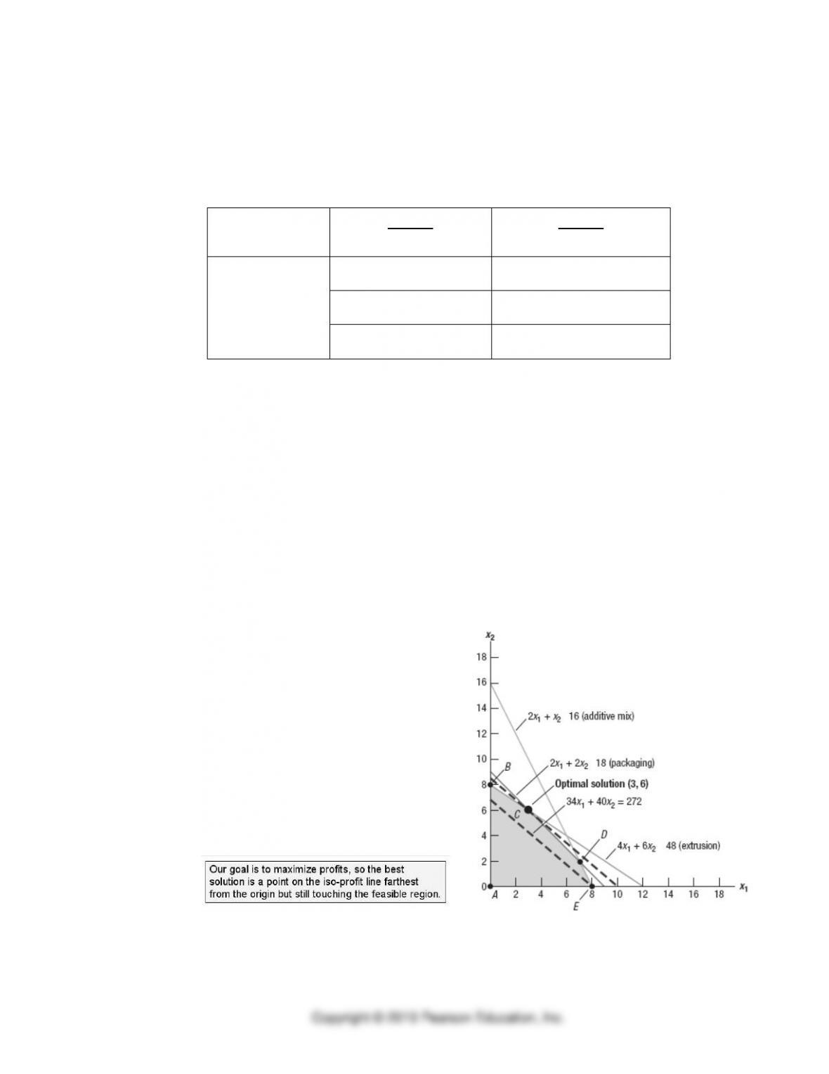
• Example D.4: Stratton Company
Step 1
4x1 + 6x2 = 48 (extrusion)
2x1 + 2x2 = 18 (packaging)
4x1 + 6x2 = 48
– (4x1 + 4x2 = 36)
2x2 =
x2 =
Step 2:
4x1 + 6(6) = 48
x1 =
Total Profit = 34( ) + 40( ) = $342
• Application D.4: Step e for Crandon Manufacturing.

Solve algebraically, with two equations and two unknowns
2 x1 + 1 x2 4000 (fabrication)
1 x1 + 2 x2 5000 (assembly)
x1 = ______
x2 = ______
Optimal Z: $900 (____) + $600 (_____) = _________
3. Slack and surplus variables
a. Binding constraint
b. Slack variables
c. Surplus variables
d. Solving for slack and surplus variables
• Application D.5: Slack Variables for Crandon Manufacturing.
The constraints are:
2x1 + 1x2 ≤ 4,000 (Fabrication)
1x1 + 2x2 ≤ 5,000 (Assembly)
1x1 + 1x2 ≤ 3,500 (Demand)
Find the slack variables at the optimal solution (1000, 2000).
Slack in fabrication:
Slack in assembly:
Slack in demand:
4. Sensitivity Analysis
a. Rarely are the parameters in the objective function and constraints known with certainty.
b. Four basic types of sensitivity analysis
Term
Definition
Reduced cost
Shadow price
Range of optimality
Range of feasibility
4. Computer Analysis
1. Simplex method
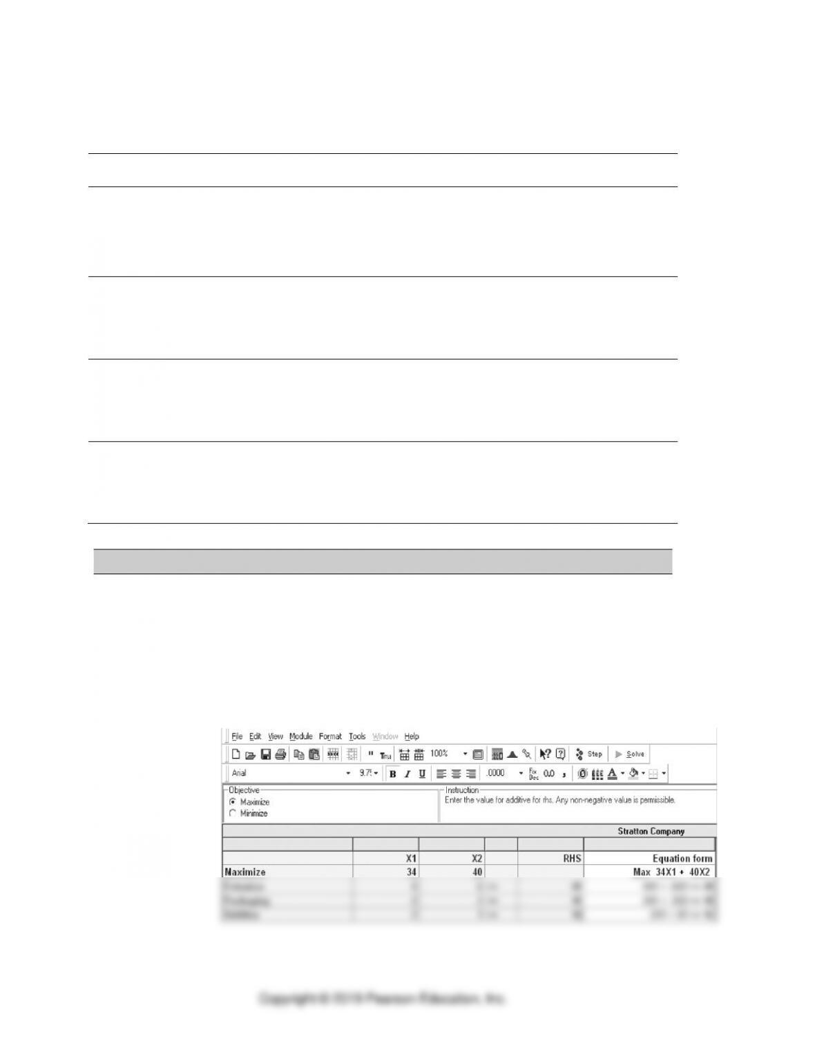
2. Computer Output for Stratton Company (from POMS for Windows)
a. Data Entry Screen
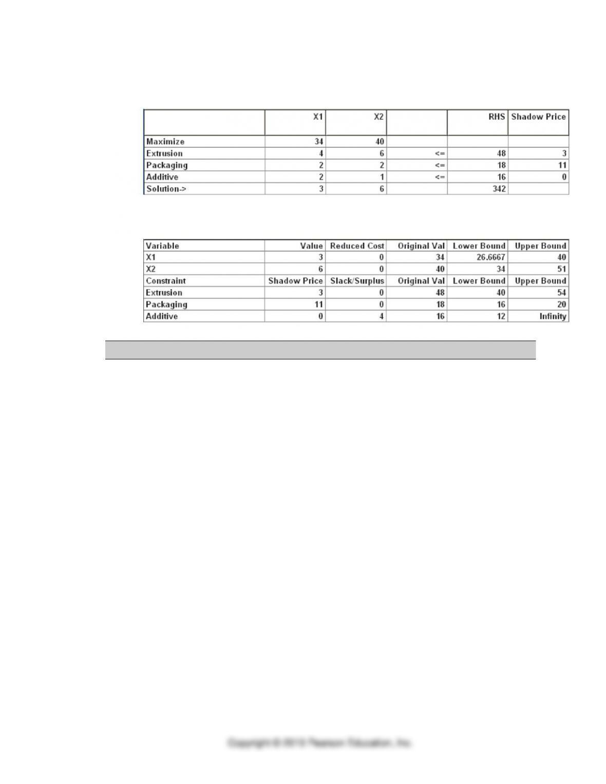
b. Results Screen
c. Ranging Screen
5. The Transportation Method
1. The transportation problem is a special case of linear programming, represented as a standard
table or tableau
a. Rows
b. Columns
c. Cells
2. Transportation method for Sales and Operations Planning
a. Balances:
b. Helpful in determining:
c. Based on several assumptions:
•
•
•
d. Example D.6 on Tru-Rainbow Company (Using POMS for Windows)
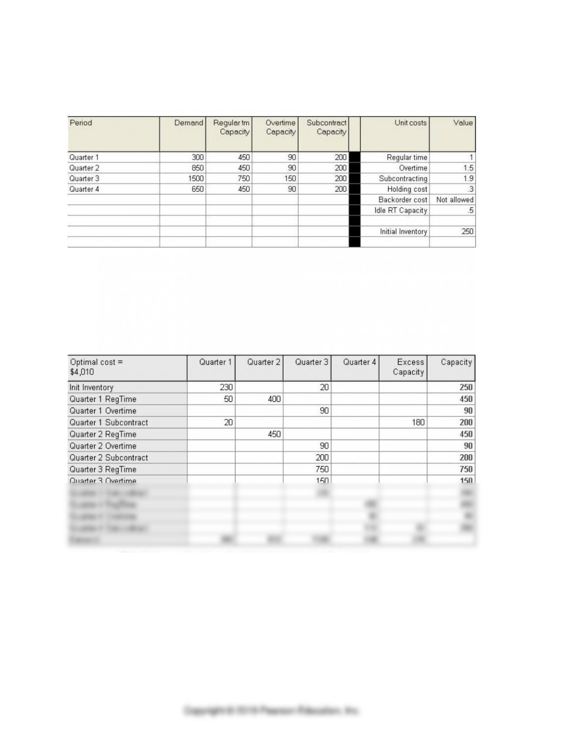
Data Table
* Note how desire for ending inventory of 300,000 gallons, with demand for quarter 4 being
350,000 gallons.
Transportation Method (Production Planning) Results
• Calculating production and anticipation inventory by period
• Calculating costs
e. Application D.6: The Transportation Method of Production Planning
The Bull Grin Company makes an animal-feed supplement. Sales are seasonal, but Bull
Grin’s customers refuse to stockpile the supplement during slack sales periods; they insist on
shipments according to their schedules to stockpile the supplement during slack sales periods
and won’t accept backorders. The supply options that they use, in addition to workforce
variation, are regular time, overtime, subcontracting, and anticipation inventory. Backorders
are not allowed.
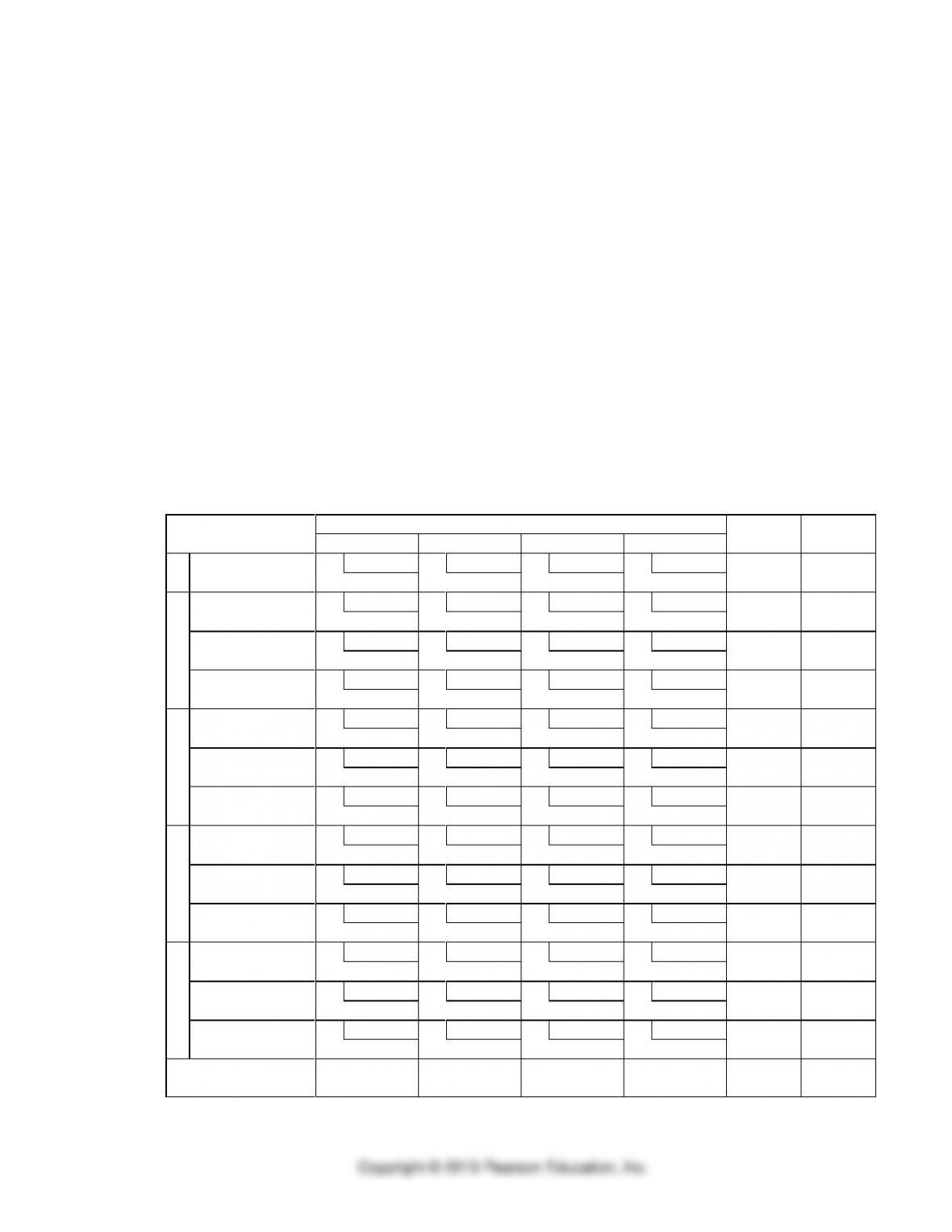
Complete the tableau given below by entering the cost per pound produced with each
production alternative to meet demand in each period. Bull Grin employs workers who
produce 1,000 pounds of supplement for $830 on regular time and $910 on over-time.
Holding 1000 pounds of feed supplement in inventory per quarter costs $100. There is no
cost for unused regular-time, overtime or subcontracting capacity.
Quarter
Unused
Total
Alternatives
1
2
3
4
Capacity
Capacity
Beginning
$0
$100
$200
$300
Inventory
40
0
Regular
$830
$930
$1,030
$1,130
Time
90
220
–
80
–
1
Overtime
$910
$1,010
$1,110
$1,210
–
–
20
–
–
Subcontract
$1,000
$1,100
$1,200
$1,300
–
–
–
–
30
Regular
$99,999
Time
180
220
–
2
Overtime
$99,999
20
–
Subcontract
$99,999
30
–
Regular
$99,999
Time
460
–
3
Overtime
$99,999
20
–
Subcontract
$99,999
30
–
Regular
$99,999
Time
380
–
380
4
Overtime
$99,999
20
–
20
Subcontract
$99,999
30
–
30
Demand
130
30
1870
Now enter data for the capacity column of the tableau (final column to right). For simplicity,
enter the data as thousands of pounds. The workforce plan being investigating now would
provide regular-time capacities (in 000’s pounds) of 390 in quarter 1, 400 in quarter 2, 460 in
quarter 3, and 380 in quarter 4. Overtime is limited to production of a total of 20,000 pounds
per quarter, and subcontractor capacity to only 30,000 pounds per quarter. The current
inventory level is 40,000 pounds.
Next enter the data for the demand row (last row in the tableau). The demand forecasts (in
000’s pounds) are 130 in quarter 1, 400 in quarter 2, 800 in quarter 3, and 470 in quarter 4.
Management wants 40,000 pounds available at the end the year. NOTE: Fourth-quarter
demand should be increased in the demand row to allow for the desired ending inventory.
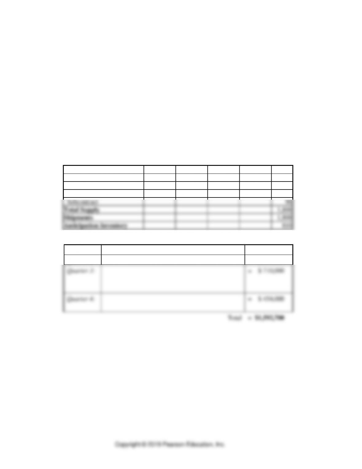
What production levels, shipments, and anticipation inventories are called for by the optimal
solution shown as bold numbers in the tableau above?
Quarter 1
Quarter 2
Quarter 3
Quarter 4
Totals
Production
Regular-time
1,630
Overtime
80
Subcontract
90
Total Supply
1,800
Shipments
1,800
Anticipation Inventory
810
What is the total cost of the optimal solution, except for the cost of hiring and layoffs?
Quarter 1:
= $ 74,700
Quarter 2:
= $ 354,000
Quarter 3:
= $ 710,000
Quarter 4:
= $ 454,000
Total
= $1,592,700