Unlock document.
This document is partially blurred.
Unlock all pages and 1 million more documents.
Get Access
Supplement
D
Linear Programming
DISCUSSION QUESTIONS
1. Overtime would relax the labor constraint, but the additional labor resource comes at a cost.
Would additional labor hours improve the solution at a rate sufficient to pay for overtime? If so,
2. For a linear programming problem, sensitivity analysis might suggest other plans that are better,
such as adding capacity at a bottleneck operation. The manager might have reservations on cost
or demand estimates, or realize that the anticipation inventories are excessive (such as when
PROBLEMS
Formulating a Linear Programming Model
1. Happy Dog Inc.
Let: X1 = the number of 5 lb. bags of Puppy Blend produced
a. The linear programming model would be:
Max Z= X1+X2+X3 (Objective Function)
Subject to: 2.5X1+1.5X2+1.0X3≤ 10,000 (Chicken availability constraint)
b. For this formulation, the objective function would include the profit per bag of food as a
coefficient. The constraints would remain unchanged.
⚫ PART 2 ⚫ Managing Customer Demand
D-2
Max Z= 1.00X1+1.25X2+2.00X3 (Objective Function)
2. Amazing Dairy
Let: X1 = the number of 10 lb. containers of Yogurt produced
The linear programming model would be:
Max Z= 15.00X1+20.00X2+35.00X3 +12.50X4 (Objective Function)
Subject to: 15X1+10X2+15X3+5X4≤ 2,400 (Machine 1 availability constraint)
25X1+10X2+15X3+5X4≤ 2,400 (Machine 2 availability constraint)
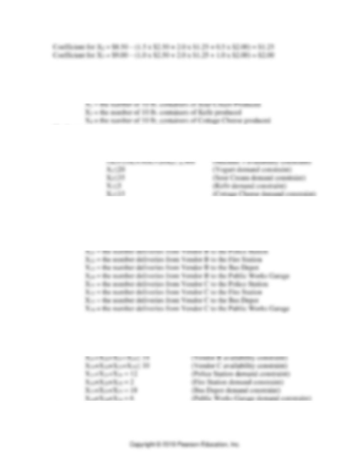
3. Lexington
Let: X11 = the number deliveries from Vendor A to the Police Station
X12 = the number deliveries from Vendor A to the Fire Station
X13 = the number deliveries from Vendor A to the Bus Depot
X14 = the number deliveries from Vendor A to the Public Works Garage
The linear programming model would be:
Min Z= 500X11+525X12+550X13 +600X14+350X21+425X22+450X23
+575X24+400X31+375X32+625X33 +475X34 (Objective Function)
Subject to: X11+X12+X13+X14≤ 20 (Vendor A availability constraint)
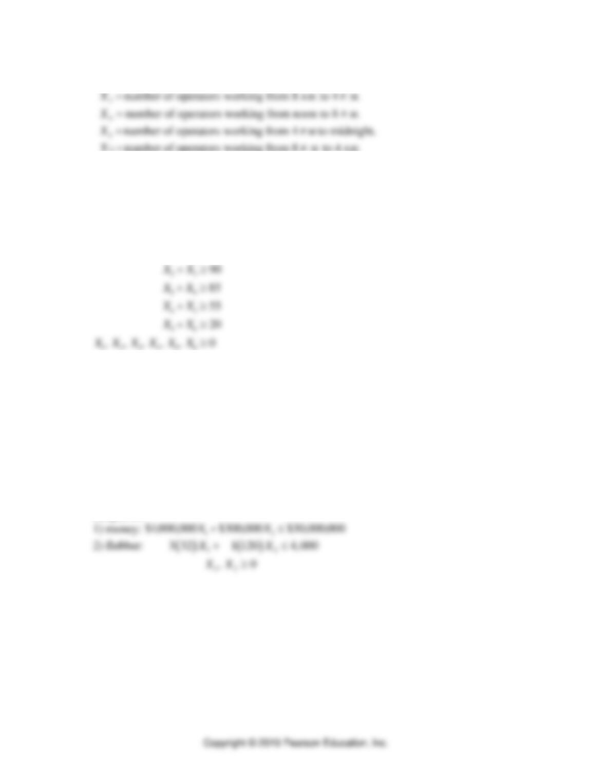
4. JPMorgan Chase
Let:
1
X=
number of operators working from midnight to 8 A.M.
Linear Programming ⚫ SUPPLEMENT D ⚫
D-3
2
X=
number of operators working from 4 A.M. to noon.
5
6
X=
number of operators working from 8 P. M. to 4 A.M.
Minimize:
ZXXXXXX =+++++ 654321
Subject to:
X X
X X
X X
X X
X X
X X X X X X
1 6
1 2
2 3
3 4
45
56
1 2 3 4 56
4
6
90
55
20
0
+
+
+
+
+
, , , , ,
Graphic Analysis
5. Sports Shoe Company
Definition of decision variables:
X1=
number of basketball teams sponsored
X2=
number of football teams sponsored
a. Objective function and constraints
Maximize:
1 1
1 2
X X+
Subject to:
12
⚫ PART 2 ⚫ Managing Customer Demand
D-4
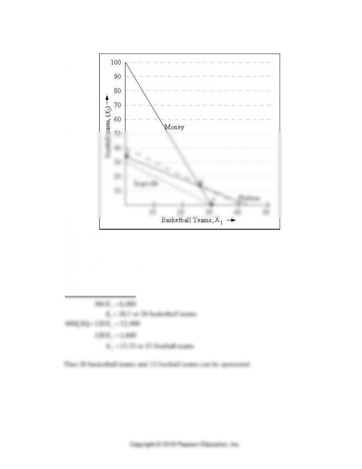
b. Graphical analysis. The optimal solution occurs at point B.
c. The optimal solution at corner point B occurs at the intersection of the money and flubber
constraints. This appears to be at coordinates (26, 14). To algebraically find the intersection
of the money and flubber constraints, we multiply the money constraint by 0.0004, and then
subtract the flubber constraint from the money constraint.
12
12
400 120 12,000
96 120 4,000
304 8,000
XX
XX
X
+=
− − = −
=
X126 3=.
or 26 basketball teams
( )
2
2
2
400 26 120 12, 000
120 1,600
13.33 or 13 football teams
X
X
X
+=
=
=
Thus 26 basketball teams and 13 football teams can be sponsored.
Linear Programming ⚫ SUPPLEMENT D ⚫
D-5
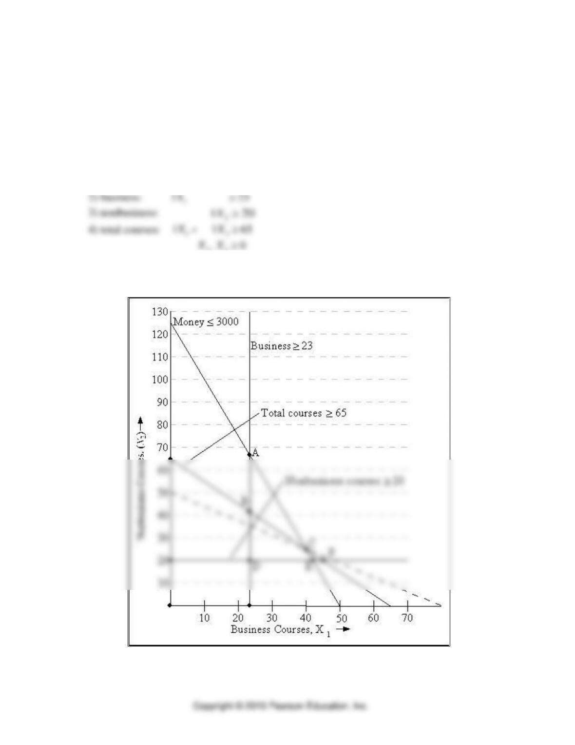
6. Nowledge College (minimize hours of study)
Definition of decision variables:
X1=
number of business courses
X2=
number of nonbusiness courses
a. Objective function and constraints
Minimize:
120 200
1 2
X X+
Subject to:
1) money:
$60 $24 $3,X X
1 2 000+
12
b. Graphic analysis. Feasible region is defined by points A, B, and C. We see visually from the
dashed iso-cost line that corner point C minimizes hours of study.
⚫ PART 2 ⚫ Managing Customer Demand
D-6
c. Optimal solution is at corner point C, which lies at the intersection of the money and total
courses constraints. This appears to be in the neighborhood of coordinates (40, 25). To
algebraically find the intersection of these two constraints, we multiply the total courses
constraint by 24, and then subtract it from the money constraint.
60X1+ 24 X2 = 3,000
Substituting X1 into the money constraint, we get
60 (40) + 24 X2 = 3,000
Thus, the optimal solution that minimizes the total hours of study is 40 business courses and
25 nonbusiness courses.
d. Neither the number of business classes nor number of nonbusiness classes is binding the
optimal solution. The surplus in business classes is 17 units, or:
1 (40) − S2 = 23
S2 = 17
The surplus in the constraint for nonbusiness classes is 5 units, or:
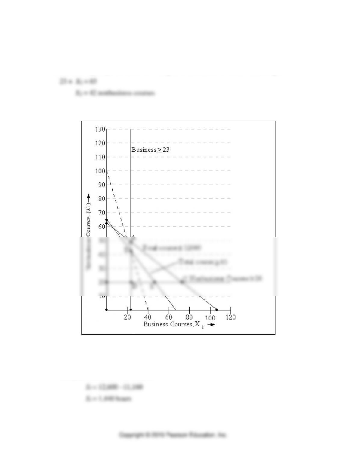
7. Nowledge College (minimize cost of books)
Definition of decision variables:
X1=
number of business courses
X2=
number of nonbusiness courses
a. Objective function and constraints
Minimize:
12
60 24XX
+
Subject to:
1) hours:
12
120 200 12, 600+XX
12
Linear Programming ⚫ SUPPLEMENT D ⚫
D-7
Graphic analysis is shown following. The feasible region is defined by corner points A, B,
C, and E. The graph shows that corner point B minimizes the total cost, which is at the
intersection of the business and total courses constraints. When the business constraint
holds as an equality, X1 = 23. Substituting into the total courses constraint, we get
Thus, the optimal solution is X1 = 23 and X2 = 42.
b. The study time limitation and number of nonbusiness classes are not binding, with the first
one having a nonzero slack variable and the second a nonzero surplus variable. The slack in
the study time constraint is 1,440 hours, or
120 (23) + 200(42) + S1 = 12,600
⚫ PART 2 ⚫ Managing Customer Demand
D-8
The surplus in the constraint for nonbusiness classes is 22 units, or
42 − S3 = 20
S3 = 22 units
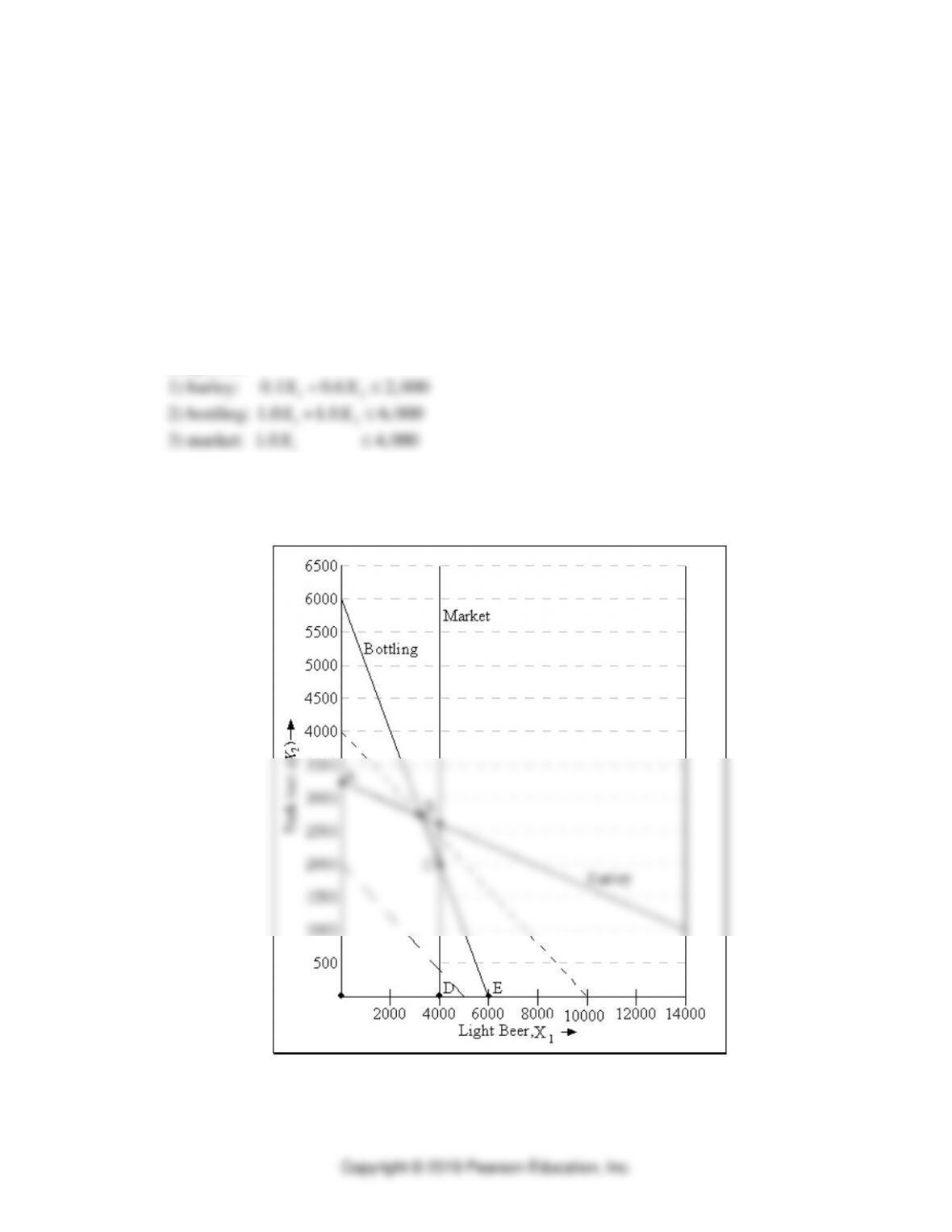
8. Mile-High Microbrewery
Definition of decision variables:
X1=
bottles of light beer
X2=
bottles of dark beer
Objective function and constraints:
Maximize:
$0.$0.20 50
1 2
X X+
Subject to:
1
a. Graphical method
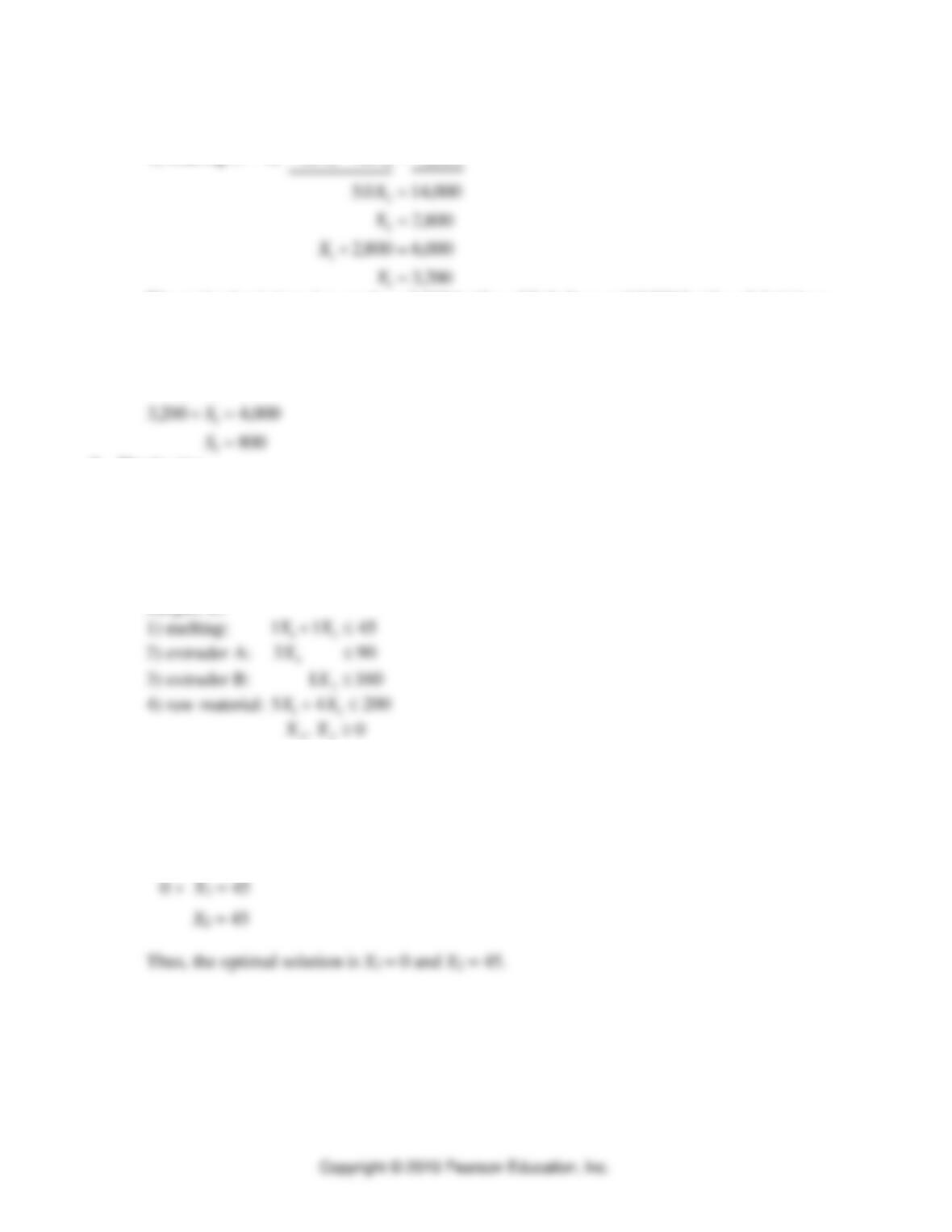
As shown following, the feasible region is defined by 0-A-B-C-D-0. The optimal solution is
at point B, the intersection between the barley constraint and the bottling constraint.
Solving for the point of intersection, we get:
Linear Programming ⚫ SUPPLEMENT D ⚫
D-9
110 10 6 0 20 000
2 1 10 10 6 000
5 0 14 000
2800
2800 6000
3200
1 2
1 2
2
2
1
1
) : . . ,
) : . . ,
. ,
,
, ,
,
barley
bottling
+ =
− − − = −
=
=
+ =
=
( )
( )
X X
X X
X
X
X
X
The optimal solution si to produce 3,200 bottles of light beer and 2,800 bottles of dark beer.
b. Only the market constraint has slack, because the other two constraints are binding. There
are 800 bottles of slack in the market constraint for light beer.
X S
S
1 3
3
3
4000
800
+ =
=
,
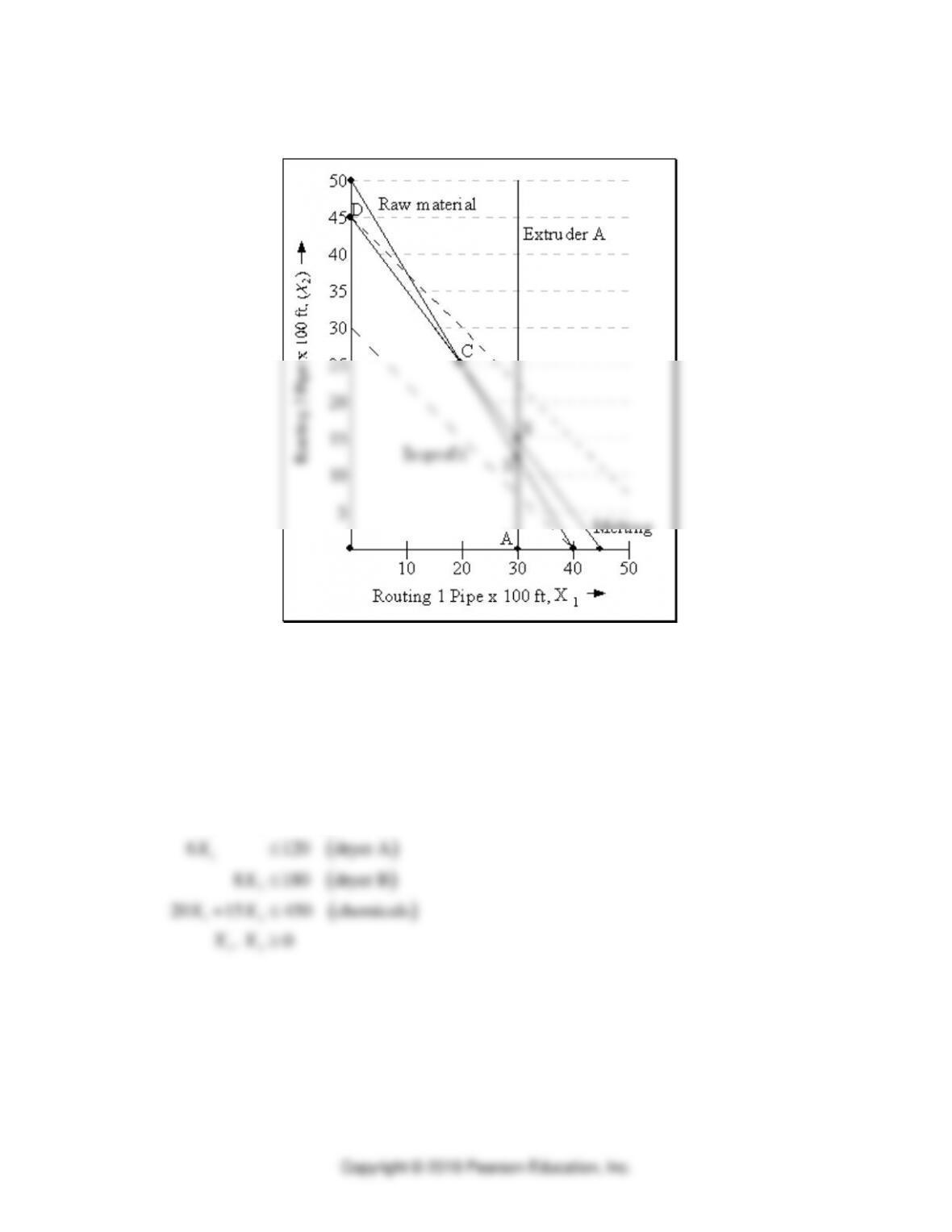
9. Plastic pipe
Definition of decision variables
X1=
hundreds of feet of pipe, routing 1
X2=
hundreds of feet of pipe, routing 2
a. Objective function and constraints
Maximize:
12
$60 $80X X Z
+=
Subject to:
⚫ PART 2 ⚫ Managing Customer Demand
D-10
c. Max
( )
$80 45 $3,600Z==
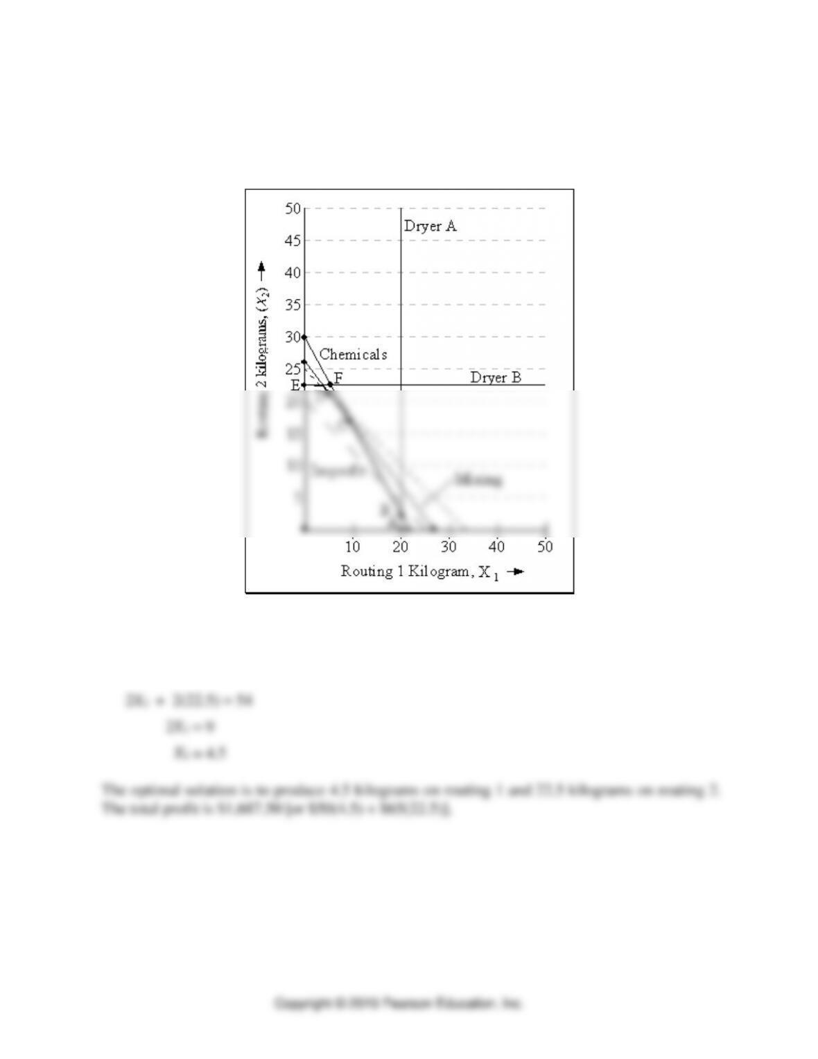
10. Manufacturer of textile dyes
a. Let
X1=
amount of dye produced on routing 1, measured in kilograms, and
2
X=
amount of dye produced on routing 2, measured in kilograms.
Then the formulation becomes
Maximize:
$50 $65X X
1 2
+
Subject to:
( )
( )
( )
12
1
2
12
12
2 2 54 mixing
6 120 dryer A
20 15 450 chemicals
, 0
XX
X
XX
XX
+
+
Linear Programming ⚫ SUPPLEMENT D ⚫
D-11
b. The graphical analysis is shown following, The feasible region is defined by corner points
A, B, C, D, E, and 0. The graph shows that corner point D maximizes profits, where the
mixing and dryer B constraints intersect. Solving first for X2 when the dryer B constraint
holds as an equality, we get
8X2 = 180
X2 = 22.5
Substituting into the mixing constraint, we get
⚫ PART 2 ⚫ Managing Customer Demand
D-12
c. Point D is the intersection of the Dryer B and the Mixing constraint. There is slack in the Dryer
A and the Chemicals constraints. There is slack in the Dryer A and the Chemicals constraints.
The Dryer A constraint has 93 hours of slack, or
6(4.5) + S2 = 120
S2 = 93
The Chemicals constraint has 22.5 hours of slack, or
Computer Analysis
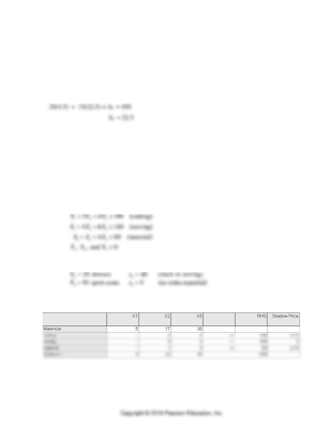
11. Trim-Look Company
a. Let
X1=
number of skirts produced
X2=
number of dresses produced
X3=
number of sport coats produced
Then the model formulation becomes:
Maximize:
$5 $17 $30X X X
1 2 3
+ +
Subject to:
X X X
X X X
X X X
X X X
1 2 3
1 2 3
1 2 3
1 2 3
3 4 100
4 6 180
460
0
+ + ( )
+ + ( )
+ +
( )
cutting
sewing
material
and , ,
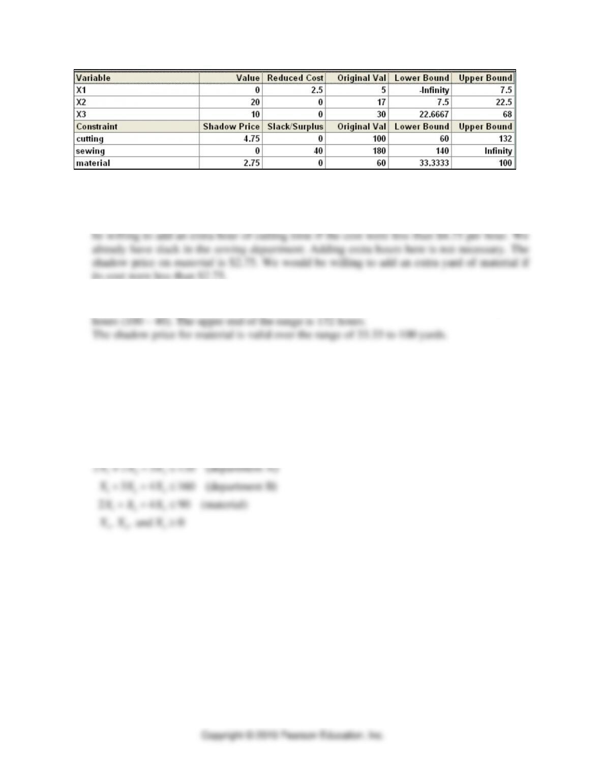
b. The optimal solution is:
X10=
skirts
s10=
(no slack in cutting)
The total profit is $640. These results are confirmed by the following two screens from the
Linear Programming module in POM for Windows:
Linear Programming ⚫ SUPPLEMENT D ⚫
D-13
12. Refer to the computer output for Problem 11 provided above.
a. The shadow price on cutting time is $4.75. This means that an additional hour of cutting
time (if it could be obtained for free) will generate an additional $4.75 in profits. We would
its cost were less than $2.75.
b. Range of feasibility.
The cutting department currently has 100 hours of capacity. The lower end of the range is 60
13. Polly Astaire
a. Let
X1=
number of shirts produced
X2=
number of shorts produced
X3=
number of pants produced
Then the formulation becomes
Maximize:
$10 $10 $23X X X
1 2 3
+ +
Subject to:
2 2 3 120
3 4 160
2 4 90
0
1 2 3
1 2 3
1 2 3
1 2 3
X X X
X X X
X X X
X X X
+ + ( )
+ + ( )
+ +
( )
department A
department B
material
and , ,
⚫ PART 2 ⚫ Managing Customer Demand
D-14
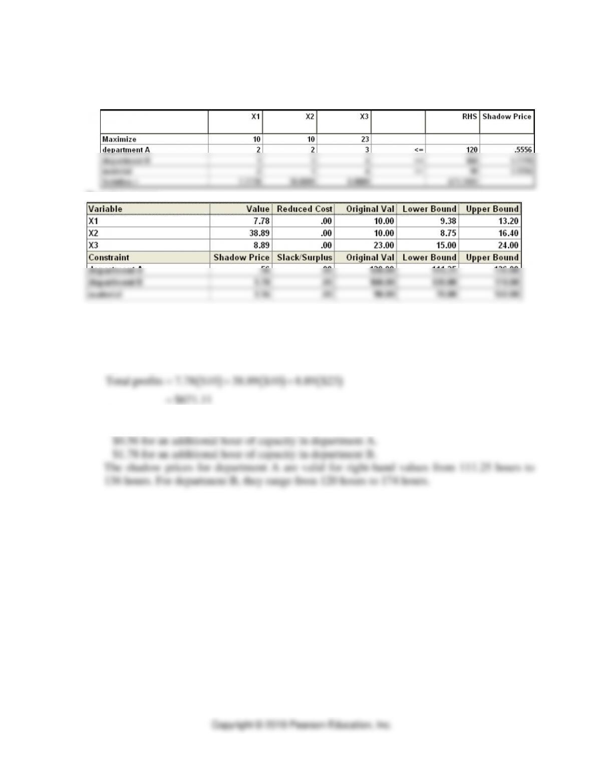
b. Using POM for Windows, we get:
Results screen
Ranging screen
Based on this output, we conclude that the optimal solution is:
X1778=.
shirts
X238 89=.
shorts
X3889=.
pants
( ) ( ) ( )
Total profits 7.78 $10 38.89 $10 8.89 $23
$671.11
= + +
=
c. There is 0 slack in all three constraints. All three resources are fully utilized. Referring to
the shadow prices, Polly Astaire would pay
Linear Programming ⚫ SUPPLEMENT D ⚫
D-15
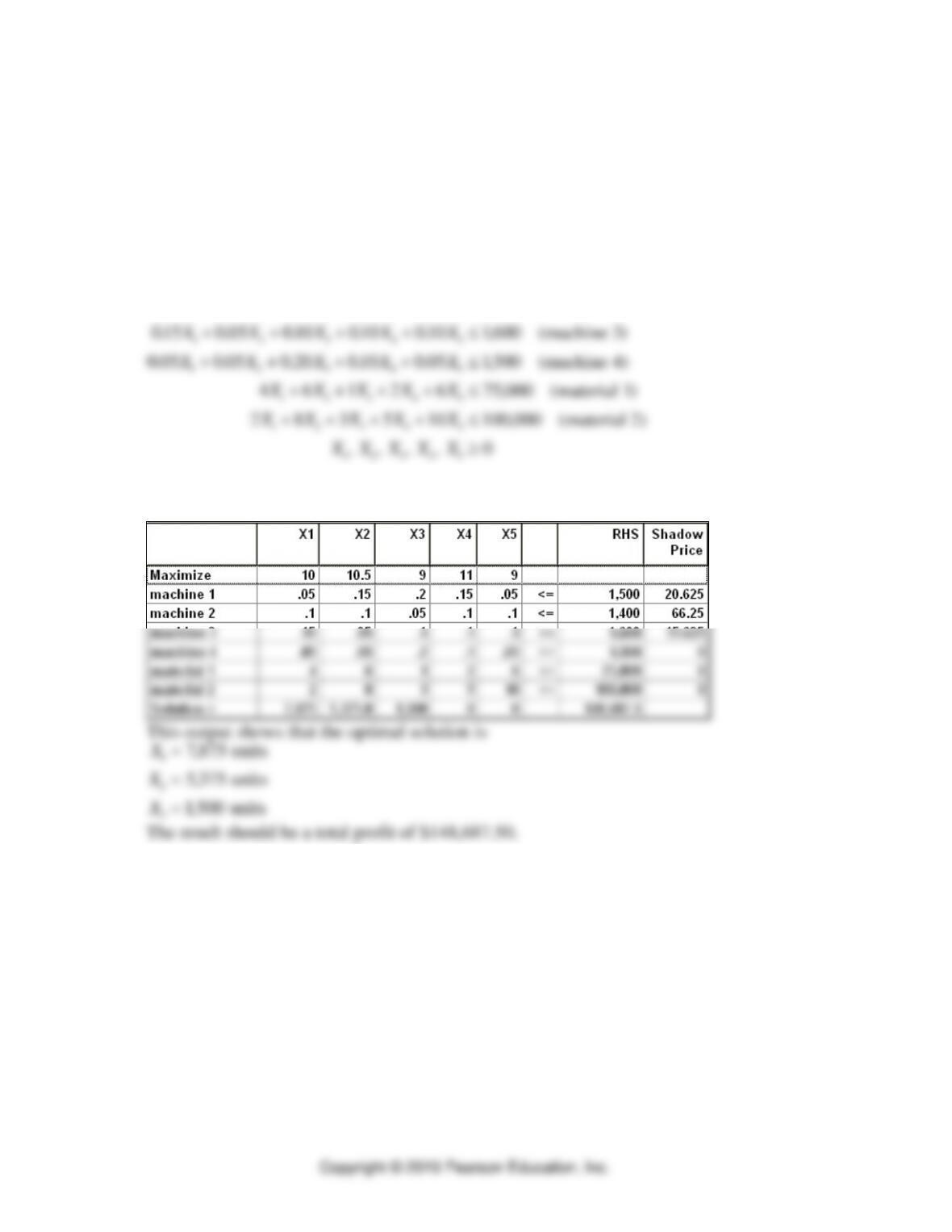
14. Butterfield Company
a. Let Xj be the number of knife j (j = A, B, C, D, and E) produced. Calculate the profit on each
knife by deducting the appropriate material costs from the selling price. The model
formulation becomes:
Maximize:
1 2 3 4 5
$10 $10.50 $9 $11 $9+ + + +X X X X X
Subject to:
005 015 020 015 005 1500
010 010 005 010 010 1400
015 005 010 010 010 1600
4 6 1 2 6 75 000
2 8
1 2 3 4 5
1 2 3 4 5
1 2 3 4 5
1 2 3 4 5
1 2 3 4 5
1
. . . . . ,
. . . . . ,
. . . . . ,
,
X X X X X
X X X X X
X X X X X
X X X X X
X
+ + + +
+ + + +
+ + + +
+ + + +
+
( )
( )
( )
( )
machine 1
machine 2
machine 3
material 1
X X X X
X X X X X
2 3 4 5
1 2 3 4 5
3 5 10 100 000
0
+ + +
( )
,
, , , ,
material 2
b. The computer output from POMS for Windows is:
⚫ PART 2 ⚫ Managing Customer Demand
D-16
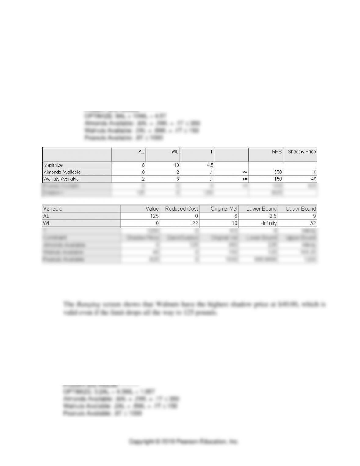
15. Nutmeg Corporation
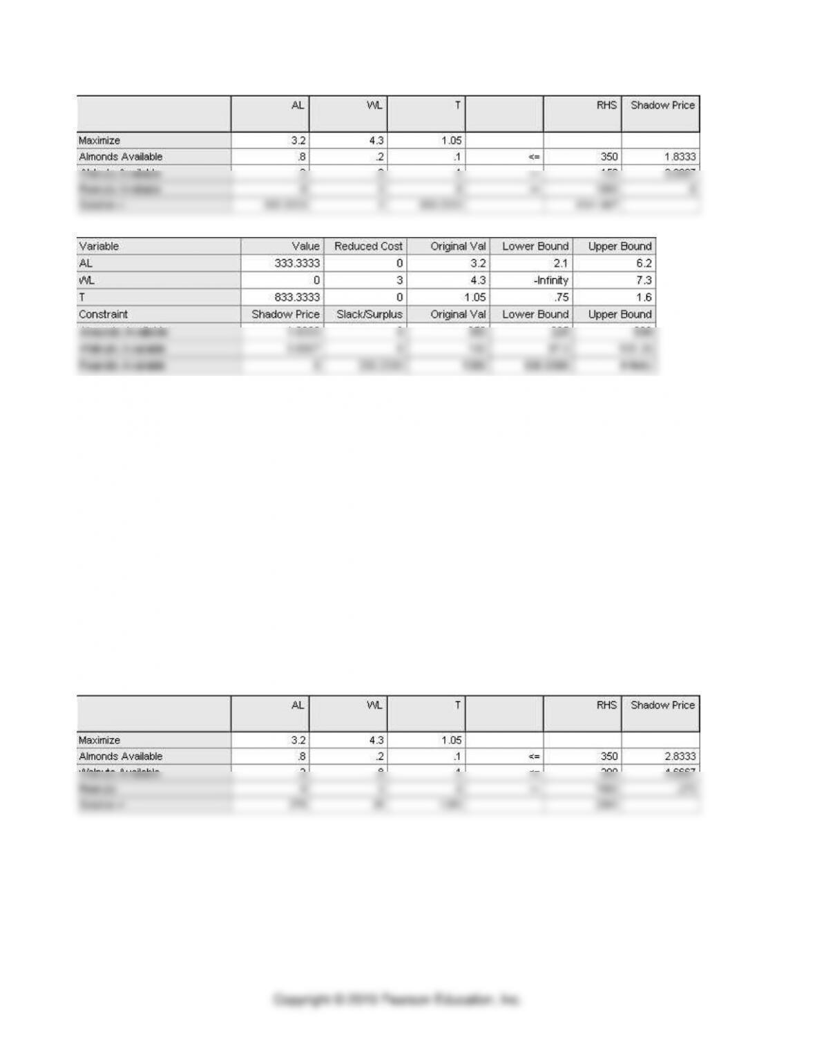
a. In order to maximize revenue, 125 cans of Almond-Lovers Mix and 1250 cans of
Thrifty Mix should be produced. Total revenue of this solution = $6,625.00
Linear programming formulation and solution using the POM for Windows Linear
Programming module, with AL for Almond Lovers, WL for Walnut Lovers, and T
for Thrifty Mix:
Objective: Maximize
Teaching point: No Walnut-Lovers would be produced, even though they have the highest
revenue. It would be unlikely to arrive at this solution without using linear programming.
b. By maximizing contribution margin, the solution will change. In order to maximize
contribution margin, 333 cans of Almond-Lovers Mix and 833 cans of Thrifty Mix should
be produced. Total contribution margin of this solution = $1940.25 (with rounding to full
cans). The linear programming formulation and solution using POM for Windows Linear
Programming module, with AL for Almond Lovers, WL for Walnut Lovers, and T for
Thrifty Mix are:
Objective: Maximize
Linear Programming ⚫ SUPPLEMENT D ⚫
D-17
Teaching point: Note that the optimal solution provides noninteger values to decision
variables. The fractional component could be viewed as production to be completed in
future periods.
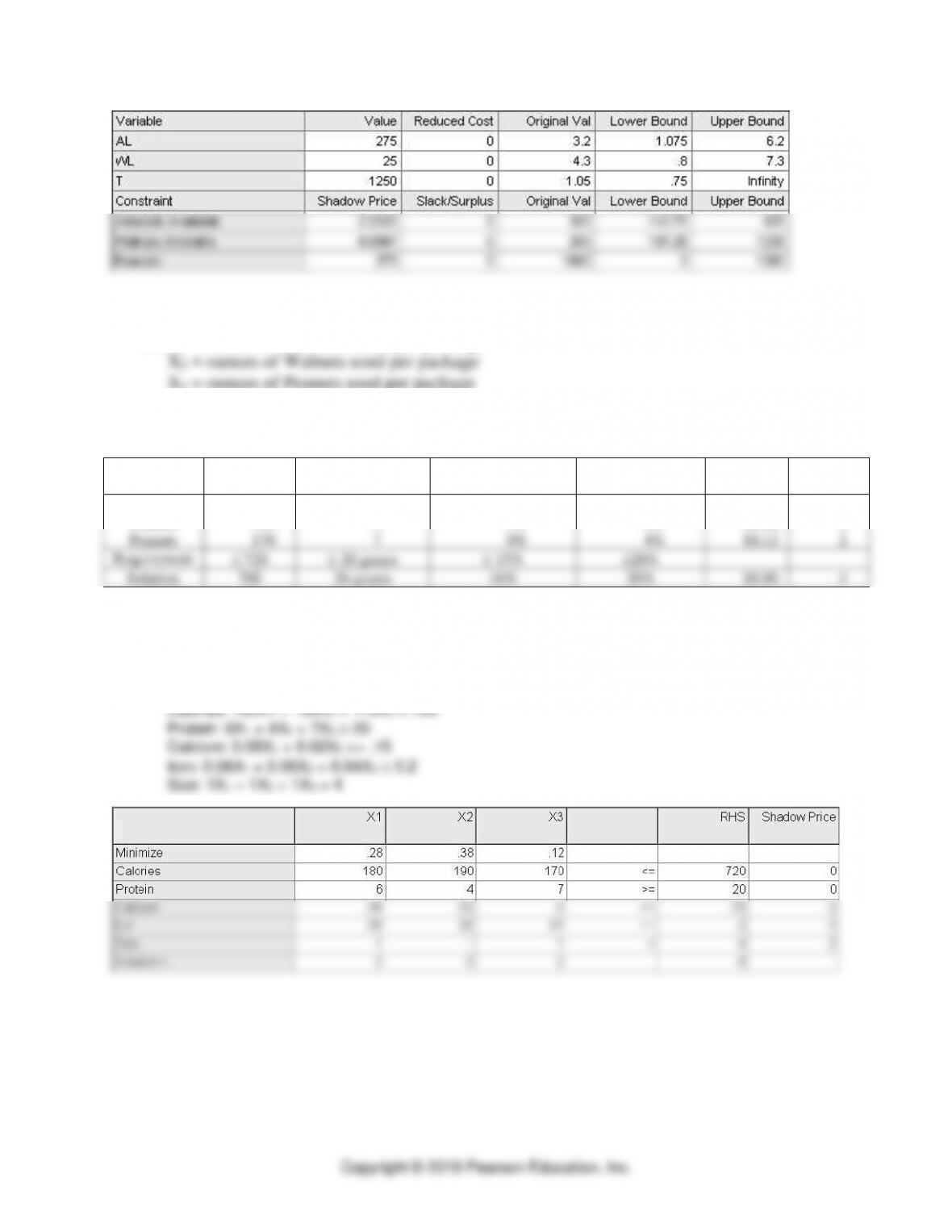
c. We know the solution will change from the shadow price of constraint 2. Given these
additional resources, 275 cans of Almond-Lovers Mix, 25 cans of Walnut-Lovers Mix and
1250 cans of Thrifty Mix should be produced. Total contribution margin of this solution =
$2,300. Linear programming formulation and solution using POM for Windows Linear
Programming module, with AL for Almond Lovers, WL for Walnut Lovers, and T for
Thrifty Mix:
Objective: Maximize
Problem and Results ----------
Maximize: 3.2AL + 4.3WL + 1.05T
Almonds Available: .8AL + .2WL + .1T 350
Walnuts Available: .2AL + .8WL + .1T 200
Peanuts Available: .8T 1000
⚫ PART 2 ⚫ Managing Customer Demand
D-18
16. Nutmeg Blending Problem
Let X1 = ounces of Almonds used per package
X3 = ounces of Peanuts used per package
a. The optimal mix is 2 ounces of almonds and 2 ounces of peanuts for a total raw material cost of
$0.80 per package.
Ingredients
Calories per
ounce
Grams of protein
per ounce
Percent ADR of
calcium per ounce
Percent ADR of
iron per ounce
Cost per
ounce
Ounces
used
Almonds
Walnuts
Peanuts
180
190
170
6
4
7
8%
2%
0%
6%
6%
4%
$0.28
$0.38
$0.12
2
0
2
Requirement
720
20 grams
15%
20%
Solution
700
26 grams
16%
20%
$0.80
4
The linear programming formulation and solution using the POM for Windows Linear
Programming module follow:
Objective: Minimize
Problem and Results ----------
Minimize: 0.28X1 + 0.38X2 + 0.12X3
Linear Programming ⚫ SUPPLEMENT D ⚫
D-19
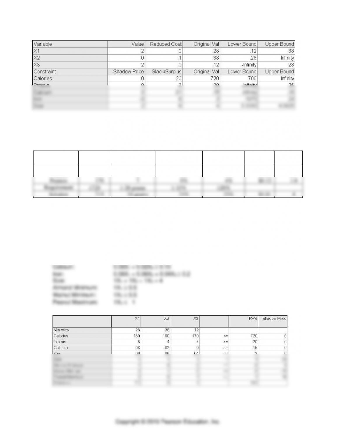
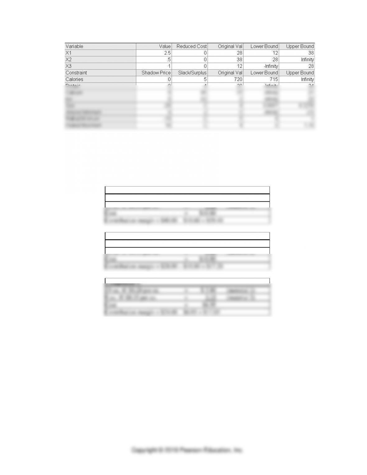
b. The solution in part a does not satisfy the marketing constraints and thereby must be
reformulated. The new optimal mix is 2.5 ounces of almonds, 0.5 ounces of walnuts and 1
ounce of peanuts for a total material cost of $1.01 per package.
Ingredients
Calories
per ounce
Grams of protein
per ounce
Percent ADR of
calcium per ounce
Percent ADR of
iron per ounce
Cost per
ounce
Ounces
used
Almonds
Walnuts
Peanuts
180
190
170
6
4
7
8%
2%
0%
6%
6%
4%
$0.28
$0.38
$0.12
2.5
0.5
1.0
Requirement
720
20 grams
15%
20%
Solution
715
24 grams
21%
22%
$1.01
4
The linear programming formulation and solution using POM for Windows Linear
Programming module follows:
Problem title: Nutmeg
Objective: Minimize
OPTIMIZE: Z=28X1 + 38X2 + 12X3
Calories: 180X1 + 190X2 + 170X3 720
Protein: 6X1 + 4X2 + 7X3 20
⚫ PART 2 ⚫ Managing Customer Demand
D-20
17. Small fabrication firm
a. First, determine the contribution margin of each component type by subtracting the material
costs from the selling price.
Component A
32 oz. @ $0.20 per oz.
=
$ 6.40
(material 1)
12 oz. @ $0.35 per oz.
=
4.20
(material 2)
Cost
=
$10.60
Contribution margin = $40.00 – $10.60 = $29.40
Component B
26 oz. @ $0.20 per oz.
=
$ 5.20
(material 1)
16 oz. @ $0.35 per oz.
=
5.60
(material 2)
Cost
=
$10.80
Contribution margin = $28.00 – $10.80 = $17.20
Component C
19 oz. @ $0.20 per oz.
=
$ 3.80
(material 1)
9 oz. @ $0.35 per oz.
=
3.15
(material 2)
Cost
=
$6.95
Contribution margin = $24.00 – $6.95 = $17.05


