Supplement
C
Special Inventory Models
PROBLEMS
Noninstantaneous Replenishment
1. Bold Vision Inc.
( )( )( )
( )
( )( )
2
ELS
2 625 52 100 1,736
.2 130 1,736 625
250,000 1.5626 500 1.25
625 toner cartridges
=−
=−
==
=
DS p
H p d
2. Sharpe Cutter
a.
( )( ) ( )
( )( )
2
ELS
2 100,000 300 450
1.20 450 400
7,071.07 3 21,213 knives
DS p
H p d
=−
=−
==
b. Total annual cost
( ) ( )
( ) ( )
2
21,213 450 400 100,000
1.20 300
2 450 21,213
$1,414.21 $1,414.22 $2,828.44
Q p d D
C H S
pQ
−
=+
−
=+
= + =
c.
( ) ( )
ELS 21,213
TBO 250 days year 250 53
100,000D
= = =
days
d. Production time/lot
ELS 21,213 47.1
450p
= = =
days
PART 2 Managing Customer Demand
C-2
3. Sud’s Bottling Company
( )( )( )
( )
( )( )
2
ELS
2 600 52 800 2400
.30 12.50 2,400 600
13,312,000 1.333 3,648.56 1.1547
4,213 cases
DS p
H p d
=−
=−
==
=
4. One-Eyed Toad
a. The production lot size that minimizes total cost is
b. The average time between orders is
c. The minimum total of setup and holding costs is
Quantity Discounts
5. Bucks Grande major-league baseball. Results from POM for Windows Software:
Demand rate(D) 17500
Setup/Ordering cost(S) 100
Holding@38%
Price Ranges From To Price
1 999 7.5
1000 4999 7.25
5000 999999 6.5
Results
Special Inventory Models ⚫ SUPPLEMENT C ⚫
C-3
Range Quantity Cost Cost Cost Cost
1 to 999
1000 to 4999 1127.13 1552.62 1552.62 126875 129980.2
5000 to 999999 5000 350 6175 113750 120275
Step 1: Calculate the EOQ at the lowest price ($6.50):
2 2(350)(50)(100) 1190.4 1190
.38(6.5)
DS
EOQ or balls
H
= = =
This solution is infeasible. We cannot buy 1190 balls at a price of $6.50 each.
Therefore, we calculate the EOQ at the next lowest price ($7.25):
2 2(350)(50)(100) 1127.13 1127
.38(7.25)
DS
EOQ or balls
H
= = =
This solution is feasible.
Step 2: Calculate total costs at the feasible EOQ and at higher discount quantities:
1127
1127
5000
5000
2
1,127 17,500
[.38($7.25)] ($100) $7.25(17,500)
2 1,127
$1,552.44 $1,552.79 $126,875.00 $129,980.23
5,000 17,500
[.38($6.50)] ($100) $6.50(17,500)
2 5,000
$6,175.00 $350.00 $11
QD
C H S PD
Q
C
C
C
C
= + +
= + +
= + + =
= + +
= + + 3,750.00 $120,275.00=
a. It is less costly on an annual basis to buy 5,000 baseballs at a time.
Demand rate(D) 17500
Setup/Ordering cost(S) 100
Holding@38%
Price Ranges From To Price
1 999 7.5
1000 4999 7.25
PART 2 Managing Customer Demand
C-4
Unit costs (PD) $113750
Total Cost $120275
6. Pfisher. The EOQ at the lowest price ($49.00) remains infeasible and the EOQ at the
next lowest price ($50.25) remains at 79 packages. The total annual cost of buying
disposable surgical packages also remains at $25,416.44 per year. Now we calculate
the annual cost associated with ordering 500 at a time:
( ) ( ) ( )
500
500
500
500 490
.2 $47.80 $64 $47.80 490
2 500
$2,390 $62.72 $23,422
$25,874.72
C
C
C
= + +
= + +
=
The quantity discount is not sufficient to cause Pfisher to buy the larger order
quantity.
7. University Bookstore
Step 1: Calculate the EOQ at the lowest price ($3.25)
( )
( )( )
2 2,500 10
2
EOQ 226.45, or 226
0.3 3.25
DS
H
= = =
Step 2: Calculate total costs at the feasible EOQ and at higher discount quantities.
( )( ) ( ) ( )( )
( )( ) ( ) ( )( )
218
2,001
2
218 2,500
0.30 3.50 $10 $3.50 2,500
2 218
$114.45 $114.67 $8,750
$8,979.12
2,001 2,500
0.30 3.25 $10 $3.25 2,500
2 2,001
$975.49 $12.49 $8,125
$9,112.98
QD
C H S PD
Q
C
C
= + +
= + +
= + +
=
= + +
= + +
=
Special Inventory Models ⚫ SUPPLEMENT C ⚫
C-5
8. Mac-in-the-Box, Inc.
Step 1: Calculate the EOQ at the lowest price ($400):
( )( )
( )
2 1,200 300
2
EOQ 106.06
.16 400
DS
H
= = =
or 106 scanners
Step 2: Calculate total costs at the feasible EOQ and at higher discount quantities.
( ) ( ) ( ) ( )
( ) ( ) ( ) ( )
95
95
95
144
144
144
2
1,200
95 .16 $500 $300 $500 1200
2 95
$3,800 $3,800 $600,000
$607,600.00
1,200
144 .16 $400 $300 $400 1200
2 144
$4,608.88 $2,500.00 $480,000
$487,108.00
QD
C H S PD
Q
C
C
C
C
C
C
= + +
= + +
= + +
=
= + +
= + +
=
The order quantity should be 144 scanners.
9. Order quantity for “an item”
Step 1: Calculate the EOQ at the lowest price ($2.00).
( )( )
( )
2 2,000 20
2
EOQ 447.2
.2 2.00
DS
H
= = =
or 447 units
PART 2 Managing Customer Demand
C-6
Step 2: Calculate total costs at the feasible EOQ and at higher discount quantities.
( ) ( ) ( ) ( )
( ) ( ) ( ) ( )
422
422
422
1000
1000
1000
2
2,000
422 .2 $2.25 $20 $2.25 2,000
2 422
$94.95 $94.79 $4,500.00
$4,689.74
2,000
1000 .2 $2.00 $20 $2.00 2000
2 1,000
$200.00 $40.00 $4,000
$4,240.00
QD
C H S PD
Q
C
C
C
C
C
C
= + +
= + +
= + +
=
= + +
= + +
=
The order quantity should be 1,000 units.
10. Bold Vision Inc.
Bold Vision Inc.’s current batch size = 625 toner cartridges
( )( )( )
( )
( )( )
2
ELS
2 625 52 100 1,736
.2 130 1,736 625
250,000 1.5626 500 1.25
625 toner cartridges
=−
=−
==
=
DS p
H p d
Yearly cost of this strategy:
400,235,4$000,225,4200,5200,5)52)(625(130100
625
)52(625
)130)(2(.
1736
6251736
2
625
2
=++=++
−
++
−
=PDS
Q
D
H
p
dpQ
C
Yearly cost including the $2.00 discount:
009,178,4$000,160,4625,1384,16)52)(625(128100
2000
)52(625
)128)(2(.
1736
6251736
2
2000
2
=++=++
−
++
−
=PDS
Q
D
H
p
dpQ
C
Yes, Bold Vision should increase their batch size to 2000 units and thereby save
Special Inventory Models ⚫ SUPPLEMENT C ⚫
C-7
One-Period Decisions
11. Downtown Health Clinic
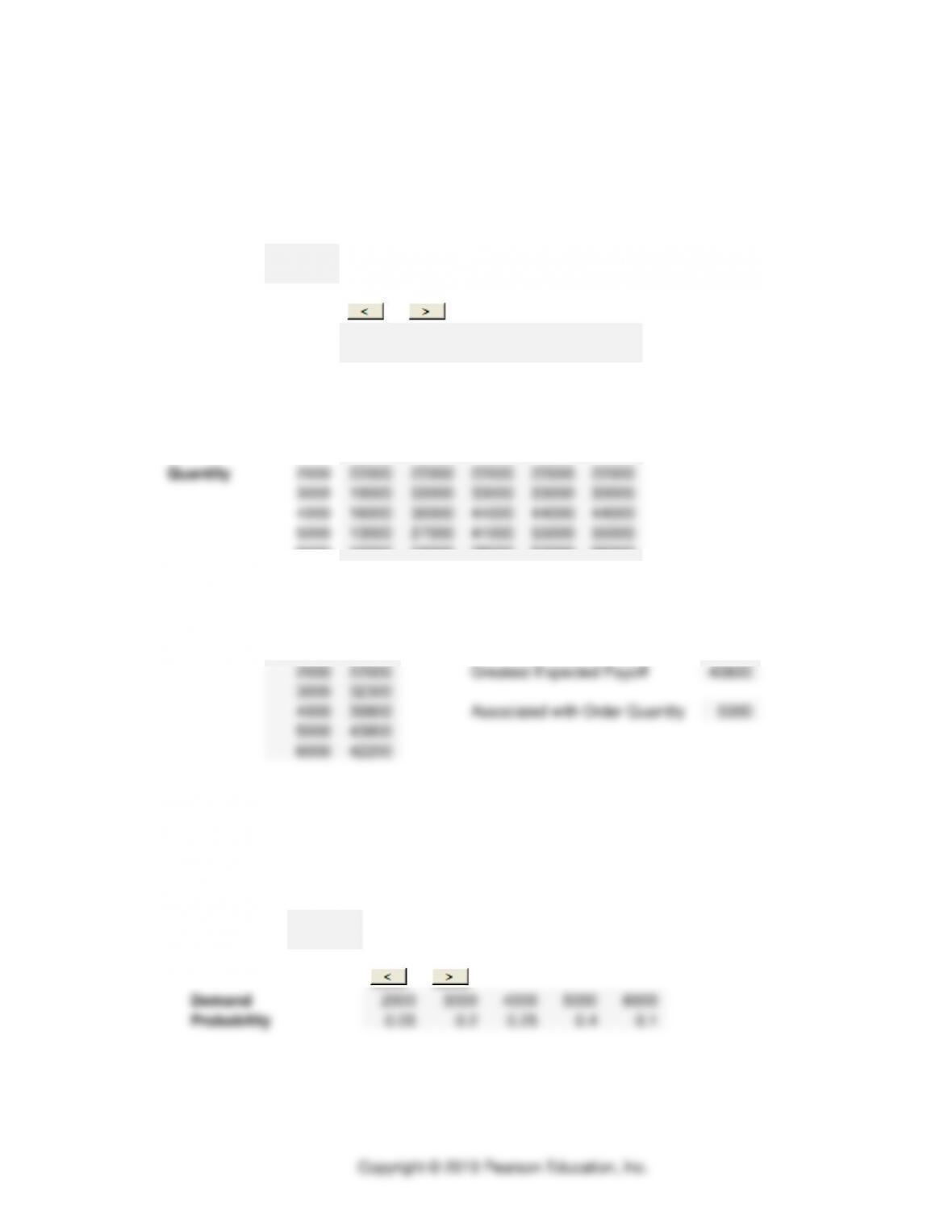
a. Order 5000 vaccines with an expected profit of $43,800. The following table
comes from the One-Period Inventory Decision Solver in OM Explorer.
Profit
$11.00
(if sold during preferred period)
Loss
$3.00
(if sold after preferred period)
Demand
2000
3000
4000
5000
6000
Probability
0.05
0.2
0.25
0.4
0.1
Payoff Table
Demand
2000
3000
4000
5000
6000
Quantity
2000
22000
22000
22000
22000
22000
3000
19000
33000
33000
33000
33000
4000
16000
30000
44000
44000
44000
5000
13000
27000
41000
55000
55000
6000
10000
24000
38000
52000
66000
Weighted Payoffs
Order
Expected
Quantity
Payoff
2000
22000
Greatest Expected Payoff
43800
3000
32300
4000
39800
Associated with Order Quantity
5000
5000
43800
6000
42200
b. If the Clinic participates in this Federal program, their profit maximizing
solution is to order 5000 vaccines with an expected profit of $32,800; an $11,000
drop in expected profitability from part (a) ($43,800 – $32,800 = $11,000). The
following table comes from the One-Period Inventory Decision Solver in OM
Explorer
Profit
$8.00
(if sold during preferred period)
Loss
$1.00
(if sold after preferred period)
Demand
2000
3000
4000
5000
6000
Probability
0.05
0.2
0.25
0.4
0.1
Payoff Table
Demand
PART 2 Managing Customer Demand
C-8
2000
3000
4000
5000
6000
Quantity
2000
16000
16000
16000
16000
16000
3000
15000
24000
24000
24000
24000
4000
14000
23000
32000
32000
32000
5000
13000
22000
31000
40000
40000
6000
12000
21000
30000
39000
48000
Weighted Payoffs
Order
Expected
Quantity
Payoff
2000
16000
Greatest Expected Payoff
32800
3000
23550
4000
29300
Associated with Order Quantity
5000
5000
32800
6000
32700
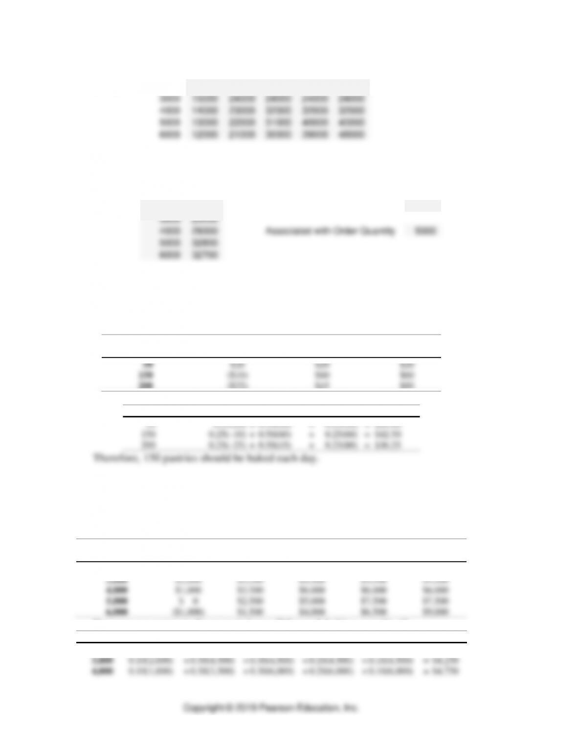
12. Dorothy’s Pastries
The following payoff matrix was constructed, where
( )
0.40 if
Payoff 0.40 0.30 if
Q Q D
D Q D Q D
=− −
D
Q
50
150
200
50
$20
$20
$20
150
($10)
$60
$60
200
($25)
$45
$80
Now we can compute the expected payoff for each baking quantity Q.
Order Quantity
Expected Payoff
50
0.25(20)
+
0.50(20)
+
0.25(20)
= $20.00
150
0.25(–10)
+
0.50(60)
+
0.25(60)
= $42.50
200
0.25(–25)
+
0.50(45)
+
0.25(80)
= $36.25
13. Aggies versus Tech
The following payoff matrix was constructed, where
( )
1.50 if
Payoff 1.50 1.00 if
Q Q D
D Q D Q D
=− −
D
Q
2,000
3,000
4,000
5,000
6,000
2,000
$3,000
$3,000
$3,000
$3,000
$3,000
3,000
$2,000
$4,500
$4,500
$4,500
$4,500
4,000
$1,000
$3,500
$6,000
$6,000
$6,000
5,000
$ 0
$2,500
$5,000
$7,500
$7,500
6,000
($1,000)
$1,500
$4,000
$6,500
$9,000
Now we can compute the expected payoff for each baking quantity Q.
Order Quantity
Expected Payoff
2,000
0.10(3,000)
+
0.30(3,000)
+
0.30(3,000)
+
0.20(3,000)
+
0.10(3,000)
=
$3,000
3,000
0.10(2,000)
+
0.30(4,500)
+
0.30(4,500)
+
0.20(4,500)
+
0.10(4,500)
=
$4,250
4,000
0.10(1,000)
+
0.30(3,500)
+
0.30(6,000)
+
0.20(6,000)
+
0.10(6,000)
=
$4,750
Special Inventory Models ⚫ SUPPLEMENT C ⚫
C-9
5,000
0.10(0)
+
0.30(2,500)
+
0.30(5,000)
+
0.20(7,500)
+
0.10(7,500)
=
$4,500
6,000
0.10(–1,000)
+
0.30(1,500)
+
0.30(4,000)
+
0.20(6,500)
+
0.10(9,000)
=
$3,750
14. The Lake Sharkey BBQ Pit
Using OM Explorer, the greatest expected payoff is $10,300 at an order quantity
of 2000 pounds.
Inputs
Solver – One-Period Inventory Decisions
Enter data in yellow shaded areas.
Profit $9.00 (if sold during preferred period)
Loss $2.00 (if sold after preferred period)
Enter the possible demands along with the probability of each occurring. Use the buttons to increase or decrease
the number of allowable demand forecasts. NOTE: Be sure to enter demand forecasts and probabilities in all tinted
cells, and be sure probabilities add up to 1.
Demand 500 1000 1500 2000 2500
Probability 0.1 0.4 0.3 0.15 0.05
Payoff Table
Demand
500 1000 1500 2000 2500
Quantity 500 4500 4500 4500 4500 4500
1000 3500 9000 9000 9000 9000
1500 2500 8000 13500 13500 13500
2000 1500 7000 12500 18000 18000
2500 500 6000 11500 17000 22500
Weighted Payoffs
Order Expected
Quantity Payoff
500 4500 Greatest Expected Payoff 10300
1000 8450
1500 10200 Associated with Order Quantity 2000
2000 10300
<
>