Supplement
C Special Inventory Models
TEACHING TIP
This chapter covers some realistic situations that require relaxation of one or more assumptions
from the EOQ: Noninstantaneous replenishment, quantity discounts, and one-period decisions.
1. Noninstantaneous Replenishment
1. Maximum cycle inventory
a. Item used or sold as it is completed, without waiting for a full lot to be completed.
b. Usual case is where production rate,
p
, exceeds the demand rate,
d
, so there is a buildup
of
( )
dp −
units per time period when both production and demand occur.
c. Both
p
and
d
expressed in same time interval, such as days.
d. Buildup continues for
pQ
days because
Q
is the lot size and
p
units are produced each
day.
e. Maximum cycle inventory is:
Imax = Q
pp−d( ) = Qp−d
p
where
=p
production rate
=d
demand rate
=Q
lot size
f. Cycle inventory is no longer
2Q
, as with the basic EOQ method, instead, it is
2
max
I
.
2. Total cost
a. Total annual cost = Annual holding cost + Annual ordering or setup cost
•
D
is annual demand and Q is lot size
•
d
is daily demand; p is daily production rate
( ) ( ) ( ) ( )
S
Q
D
H
p
dpQ
S
Q
D
H
I
C+
−
=+= 22
max
3. Economic Production Lot Size (ELS): optimal lot size
a. Derived by calculus.
b. Because the second term is greater than 1, the ELS results in a larger lot size than the
EOQ.
dp
p
H
DS
ELS −
=2
4. Use Application C.1: Noninstantaneous Replenishment to show the difference between
the ELS model and the EOQ model.
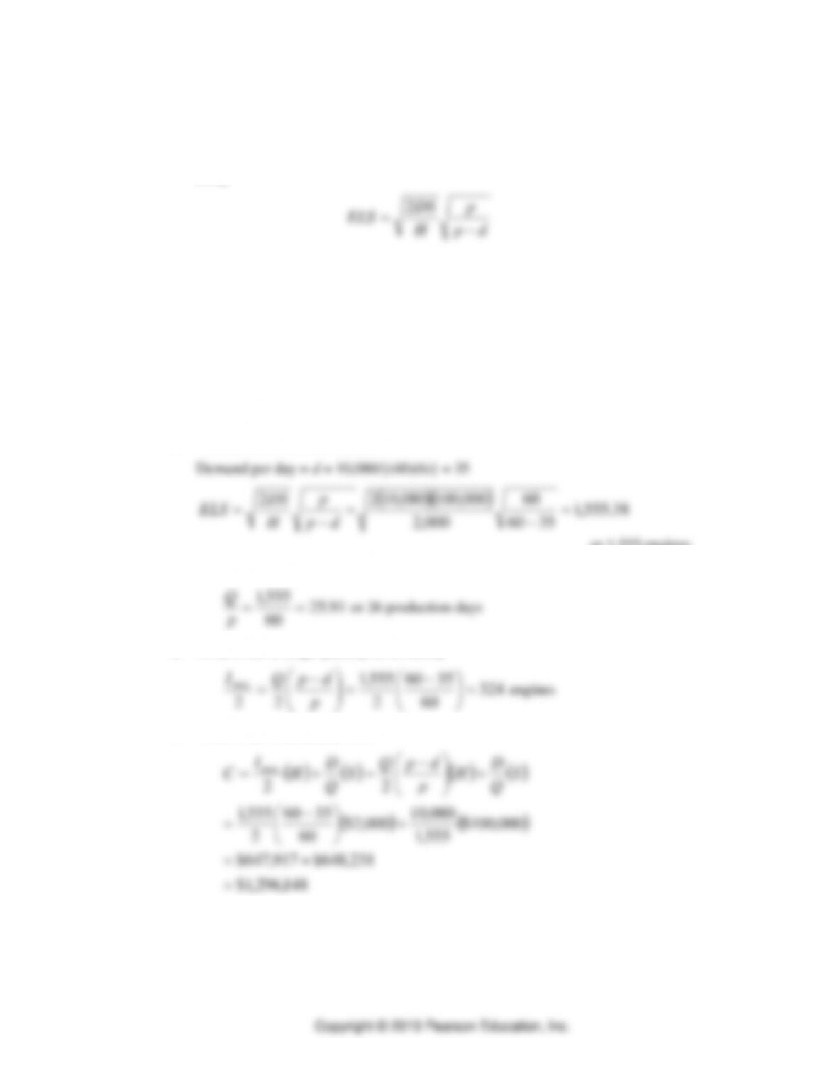
A domestic automobile manufacturer schedules 12 two-person teams to assemble 4.6 liter
DOHC V-8 engines per work day. Each team can assemble 5 engines per day. The
automobile final assembly line creates an annual demand for the DOHC engine at 10,080
units per year. The engine and automobile assembly plants operate 6 days per week, 48 weeks
per year. The engine assembly line also produces SOHC V-8 engines. The cost to switch the
production line from one type of engine to the other is $100,000. It costs $2,000 to store one
DOHC V-8 for one year.
a. What is the economic lot size?
3560
000,2
−
−
H
or 1,555 engines
b. How long is the production run?
91.25
60
555,1 ==
p
Q
or 26 production days
c. What is the average quantity in inventory
324
60
3560
2
555,1
22
max =
−
=
−
=p
dpQ
I
engines
d. What is the total annual cost?
( ) ( ) ( ) ( )
( ) ( )
148,296,1$
231,648$917,647$
000,100$
555,1
080,10
000,2$
60
3560
2
555,1
22
max
=
+=
+
−
=
+
−
=+= S
Q
D
H
p
dpQ
S
Q
D
H
I
C
5. Tutor C.1 in MyLab Operations Management provides a new example to determine the ELS.
6. Active Model C.1 in MyLab Operations Management provides additional insight on the ELS
model and its uses.
2. Quantity Discounts
1. Quantity discounts
a. There are price incentives to purchase large quantities that create pressure to maintain a
large inventory.
b. The item’s price is no longer fixed, as assumed in the EOQ
• If the order quantity is increased enough, then the price per unit is discounted
• A new approach is needed to find the best lot size. One that balances
2. Total annual cost = Annual holding costs + Annual ordering costs + Annual cost of materials
( ) ( )
PDS
Q
D
H
Q
C++= 2
where P = per unit price
a. Unit holding cost
( )
H
is usually expressed as a percentage of unit price because the
more valuable the item held in inventory, the higher its holding cost.
b. The lower the unit price
( )
P
is, the lower the unit holding cost
( )
H
is.
c. The total cost equation yields U-shape total cost curves.
• There are cost curves for each price level.
• The feasible total cost begins with the top curve, then drops down, curve by curve, at
the price breaks.
• EOQs do not necessarily produce the best lot size.
3. Two-step solution procedure to find the best lot size
a. Step 1. Beginning with lowest price, calculate the EOQ for each price level until a
feasible EOQ is found. It is feasible if it lies in the range corresponding to its price. Each
subsequent EOQ is smaller than the previous one, because
P
, and thus
H
gets larger and
because the larger
H
is in the denominator of the EOQ formula.
b. Step 2. If the first feasible EOQ found is for the lowest price level, this quantity is the
best lot size. Otherwise, calculate the total cost for the first feasible EOQ and for the
larger price break quantity at each lower price level. The quantity with the lowest total
cost is optimal.
• Finding Q with Quantity Discounts. Use Application C.2 to demonstrate the steps
for recognizing quantity discounts in making lot size decisions.
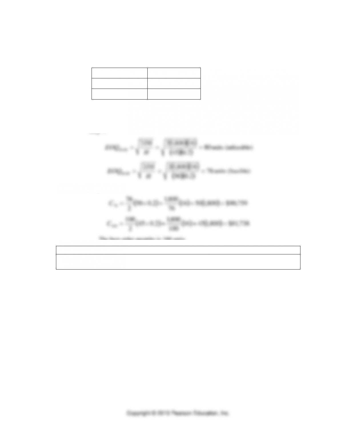
A supplier’s price schedule is:
Order Quantity
Price per Unit
0–99
$50
100 or more
45
If ordering cost is $16 per order, annual holding cost is 20 percent of the purchase price,
and annual demand is 1,800 items, what is the best order quantity?
Step 1:
( )( )
( )( )
80
2.045
16800,122
00.45 === H
DS
EOQ
units (infeasible)
( )( )
( )( )
76
2.050
16800,122
00.50 === H
DS
EOQ
units (feasible)
Step 2:
( ) ( ) ( )
759,90$800,15016
76
800,1
2.050
2
76
76 =++=C
( ) ( ) ( )
738,81$800,14516
100
800,1
2.045
2
100
100 =++=C
The best order quantity is 100 units.
TEACHING TIP
Caution: make sure students understand that the best solution is not always to choose the lowest
price per unit
4. Tutor C.2 in MyLab Operations Management provides a new example for choosing the best
order quantity when discounts are available.
5. Active Model C.2 in MyLab Operations Management provides additional insight on the
quantity discount model and its uses.
3. One-Period Decisions
1. A dilemma facing many retailers is how to handle seasonal goods. They cannot be sold at full
markup after season and cannot rush through a seasonal order to cover high demand.
2. Newsboy problem.
a. Step 1: List different demand levels and probabilities.
b. Step 2: Develop a payoff table that shows the profit for each purchase quantity,
Q
, at
each assumed demand level,
D
.
• Each row in the table represents a different order quantity and each column represents a
different demand.
• The payoff for a given quantity-demand combination depends on whether all units are
sold at the regular profit margin during the regular season, which results in two
possible cases.
If demand is high enough
( )
DQ
, then all of the cases are sold at the full profit
margin,
p
, during the regular season
( )( )
pQ== quantity Purchaseunitper Profit Payoff
If the purchase quantity exceeds the eventual demand
( )
DQ
, only
D
units are
sold at the full profit margin, and the remaining units purchased must be disposed
of at a loss,
l
, after the season.
( )
( )
DQlpD −−=
−
=seasonafter of
disposedAmount
unit
per Loss
Demand
season during
soldunit per Profit
Payoff
c. Step 3: Calculate the expected payoff of each
Q
by using the expected value decision
rule. For a specific
Q
, first multiply each payoff by its demand probability, and then add
the products.
d. Step 4: Choose the order quantity Q with the highest expected payoff.
3. One-Period Decisions. Use Solved Problem 3 to demonstrate the use of a pay-off table to
make one-period inventory decisions.
4. Tutor C.3 in MyLab Operations Management provides a new example to practice the
one-period inventory decision.
5. Active Model C.3 in MyLab Operations Management provides additional insight on the
one-period inventory decision model and its uses.