A-1
Supplement
A
Decision Making
PROBLEMS
Break-Even Analysis
1. Williams Products
a. Break-even quantity
Q
( ) = −
( )
= −
( )
=
Fixed costs Unit price Unit variable costs
units
$60,$18 $6
,
000
5000
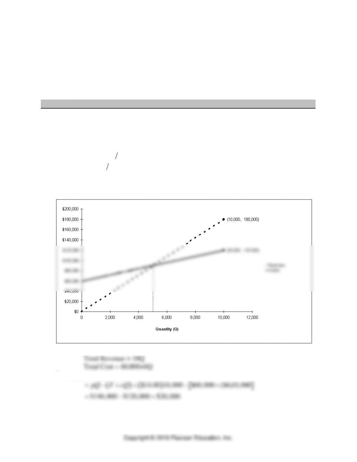
The graphic approach is shown on the following illustration, using Break-Even Analysis
Solver of OM Explorer.
Two lines must be drawn:
b. Profit = Total Revenue – Total Cost
( ) ( )
$14.00 10,000 $60,000 ($6)10,000
$140,000 $120,000 $20,000
pQ F cQ= − + = − +
=−=
c. Profit = Total Revenue – Total Cost
Decision Making
A-2
( ) ( ) ( )
$12.50 15,000 $60,000 $6 15,000
$187,500 $150,000 $37,500
pQ F cQ= − + = − +
=−=
Therefore, the strategy of using a price of $12.50 will result in a greater contribution to
profits.
d. Williams must also consider how this product fits within her existing product line from
the perspective of required technologies and distribution channels. Other marketing,
operations, and financial criteria must also be considered.
2. Jennings Company
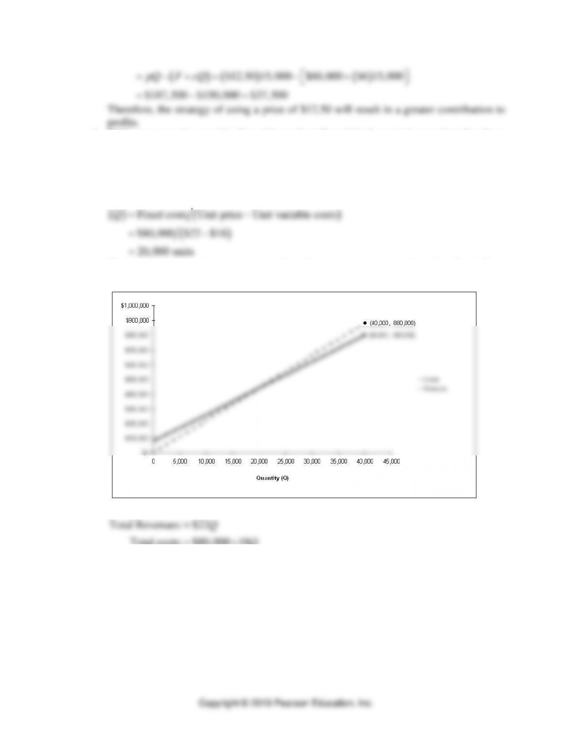
a. Break-even quantity
( ) ( )
( )
Fixed costs Unit price Unit variable costs
$80,000 $22 $18
20,000 units
Q=−
=−
=
The graphic approach is shown on the following graph created by the Break-Even
Analysis Solver.
Two lines are:
Two lines are:
Total Revenues: $22
Total costs: $80,000 18
Q
Q
=
=+
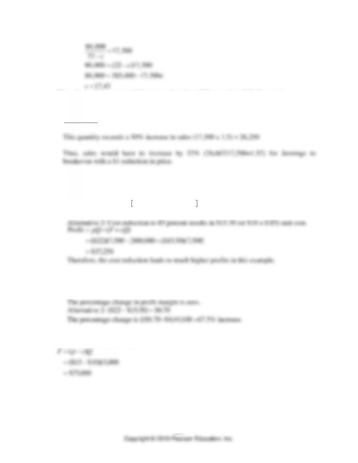
b. To calculate the new unit variable cost required to breakeven, use the breakeven equation
from part a, but solve for unit variable cost (c).
Decision Making ⚫ SUPPLEMENT A ⚫
A-3
80,000 17,500
22
80,000 (22 )17,500
80,000 385,000 17,500
17.43
cc
c
c
=
−
=−
=−
=
Thus, the variable cost would have to reduce from $18 per unit to $17.43 per unit.
c. With a $1 price decrease, the breakeven quantity would be:
80,000 26,667
(22 1) 18 =
−−
d. Alternative 1: Sales increase by 30 percent, to 22,750 units (or 17,500 x 1.3).
Profit = − +
( )
=( ) − + ( )
=
pQ FcQ
$22 ,$80,$18 ,
$11,
22 750 000 22 750
000
e. Initial unit profit is
$22 $18 $4.−
( ) =00
Alternative 1:
$22 $18 $4.−
( ) =00
3. Interactive television service
F p c Q= −
( )
= −
( )
=
$15 $10 ,
$75,
15 000
000
4. Brook Trout
Decision Making
A-4
( )
( )
$10,600 800 $6.70
$19.95
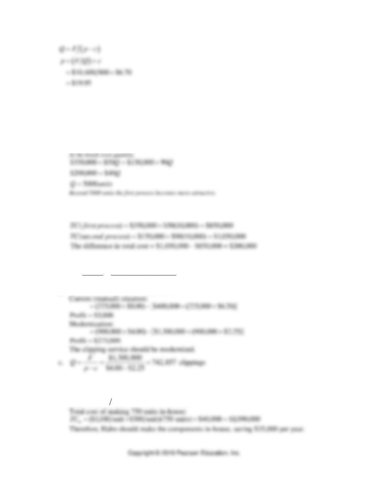
Q F p c
p F Q c
=−
=+
=+
=
5. Spartan Castings
a.
Total cost Fixed cost Variable cost=+
QprocessondTC
QprocessfirstTC
cQFTC
90$000,150$)(sec
50$000,350$)(
+=
+=
+=
b. At Q=10,000 units
000,050,1$)000,10(90$000,150$)(sec
000,850$)000,10(50$000,350$)(
=+=
=+=
processondTC
processfirstTC
The difference in total cost = $1,050,000 – $850,000 = $200,000
6. News clipping service
a.
QF F
c c
m a
a m
=−
−=−
−=
$400,$1, ,
$2.$6.,
000 300 000
25 20 227848
clippings
b.
Profit Total Revenue Total Cost= −
$4.00 $2.25
−−
7. Hahn Manufacturing
a. Total cost of buying 750 units from the supplier:
TCb=( ) =
( )
$1,$1, ,500 750 125 000unit units
Decision Making ⚫ SUPPLEMENT A ⚫
A-5
400
Q
= units
c. If the decision is to “buy,” Hahn may get a quantity discount from the supplier (we
would be ordering 750 per year instead of the current 150 per year). Just a $50 per unit
8. Techno Corporation
( )( )
Current Profit= Price Variable cost Annual Volume Annual Fixed Costs−−
.
( )( ) ( )
$10.00 $5.00 30,000 $140,000
$10,000
= − −
=
9. This problem is a thinly disguised portrayal of an actual situation faced by Tri-State G&T
Association, Inc. of Thornton, Colorado, and which is common to many other REA Utilities.
However, the costs, prices, and demands stated in the problem are fictional.
a.
F
Qpc
=−
$82,500,000 $25 $107.5 per MWH
1,000,000
F
pc
Q
= + = + =
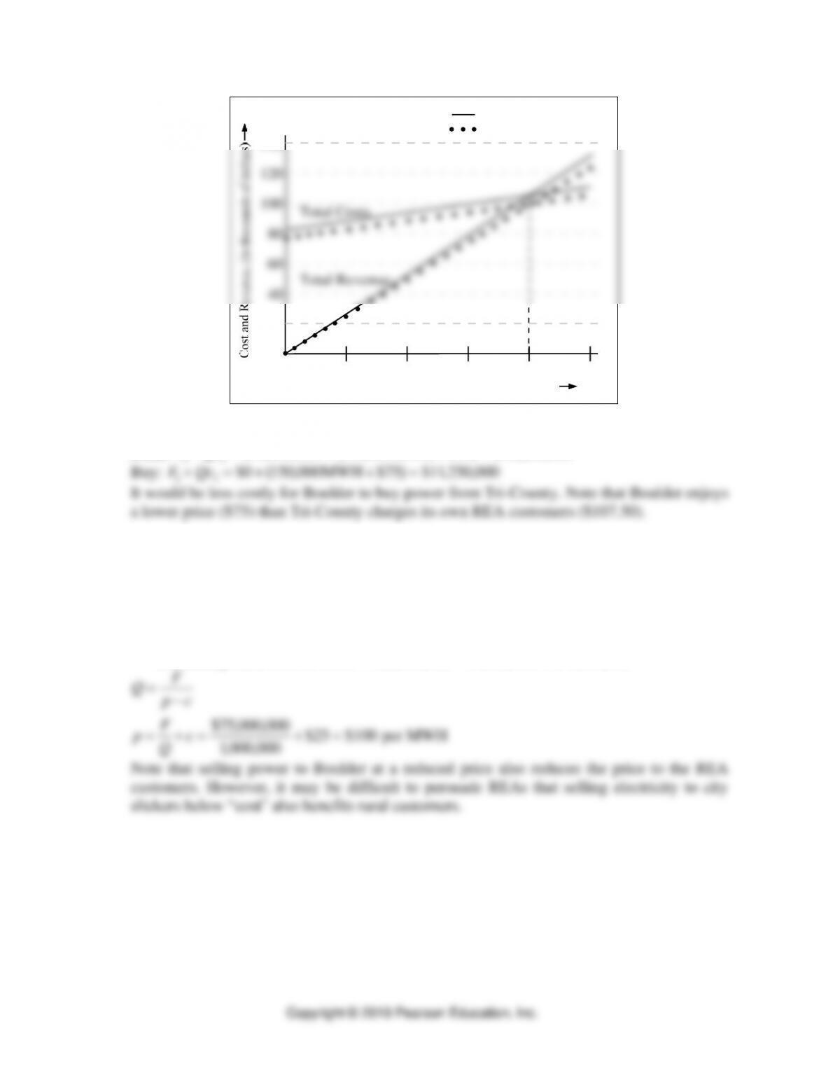
Decision Making
A-6
140
120
100
80
60
40
20
0.25 0.50 0.75 1.00 1.25
Volume, ( , in thousands of MWH)Q
Total Revenue
Total Costs
Problem 9
Problem 11
Tri-County G&T:
10. Earthquake … Build or Buy. This problem is related to problem 9.
Build:
FQc
1 1 000 000 150 000 250 000+ = +
( ) =$10, , , $35 $15, ,MWH
11. Tri-County G&T continued. This problem builds on problems 9 and 10 to show that
Tri-County’s REA customers also benefit from the bargain arrangement with Boulder.
Contribution from sales to Boulder
Remaining fixed costs to cover
= −
( )
= −
( )
=
= − =
Q p c
150 000
500 000
500 000 500 000 000 000
,$75 $25
$7, ,
$82, , $7, , $75, ,
QF
p c
pF
Qc
=−
= + = + =
$75, ,
, , $25 $100
000 000
1000 000 per MWH
Note that selling power to Boulder at a reduced price also reduces the price to the REA
customers. However, it may be difficult to persuade REAs that selling electricity to city
slickers below “cost” also benefits rural customers.
Decision Making ⚫ SUPPLEMENT A ⚫
A-7
Preference Matrix
12. Forsite Company
a. Say that each criterion (arbitrarily) receives 20 points:
Service
Calculation
Total Score
A
20 0 6 20 0 7 20 0 4 20 10 20 0 2. . . . .
( ) ( ) ( ) ( ) ( )
+ + + +
= 58
B
20 0 8 20 0 3 20 0 7 20 0 4 20 10. . . . .
( ) ( ) ( ) ( ) ( )
+ + + +
= 64
C
20 0 3 20 0 9 20 0 5 20 0 6 20 0 5. . . . .
( ) ( ) ( ) ( ) ( )
+ + + +
= 56
The best alternative is service B and the worst is service C. This relationship holds as
long as any arbitrary weight is equally applied to all performance criteria.
b. Let
x
x
x xxxx
x
x
=
=
+ + + + =
=
=
( )
point allocation to criteria 1, 3, 4, and 5
point allocation to criteria 2 ROI
points
points
points
2
2100
6100
16 7.
Product
Calculation
Total Score
A
16 7 0 6 333 0 7 16 7 0 4 16 7 10 16 7 0 2. . . . . . . . . .
( ) ( ) ( ) ( ) ( )
+ + + +
= 60.0
B
16 7 0 8 333 0 3 16 7 0 7 16 7 0 4 16 7 10. . . . . . . . . .
( ) ( ) ( ) ( ) ( )
+ + + +
= 58.4
C
( ) ( ) ( ) ( ) ( )
16.7 0.3 33.3 0.9 16.7 0.5 16.7 0.6 16.7 0.5+ + + +
= 61.7
The rank order of the services has changed to C, A, B.
13. Five new suppliers
a. Let
x
x
x
x x x x
x
x
=
=
=
+ + + =
=
=
point allocation to criteria 2 and 3
point allocation to criterion 1
point allocation to criterion 4
points
points
points
4
4
4 4 100
10 100
10
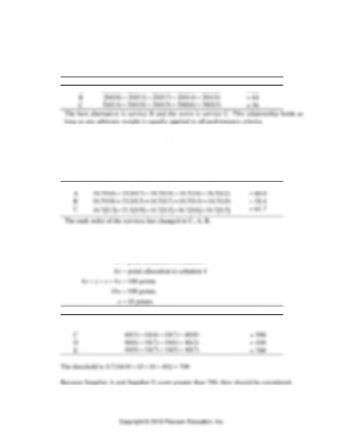
Supplier
Calculation
Total Score
A
40 8 10 3 10 9 40 7
( ) ( ) ( ) ( )
+ + +
= 720
B
40 710 810 540 6
( ) ( ) ( ) ( )
+ + +
= 650
C
40 3 10 4 10 7 40 9
( ) ( ) ( ) ( )
+ + +
= 590
D
40 6 10 7 10 6 40 2
( ) ( ) ( ) ( )
+++
= 450
E
40 910 710 540 7
( ) ( ) ( ) ( )
+ + +
= 760
b. If the factors are equally weighted:
Decision Making
A-8
Supplier
Calculation
Total Score
A
25(8+3+9+7)
= 675
B
25(7+8+5+6)
= 650
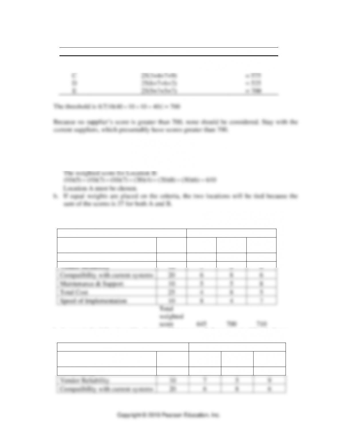
C
25(3+4+7+9)
= 575
D
25(6+7+6+2)
= 525
E
25(9+7+5+7)
= 700
14. Accel-Express Inc.
a. The weighted score for Location A:
10 8 10 7 10 4 20 7 20 4 30 7 620
( )( ) ( )( ) ( )( ) ( )( ) ( )( ) ( )( )
+ + + + + =
15. Krebs Consulting
a. As seen in the table below, Vendor C has the best rating of 710.
Rating
Performance Criterion
Factor
Weight
Software
A
Software
B
Software
C
Functionality
25
9
8
9
Vendor Reliability
10
7
5
9
Compatibility with current systems
20
6
8
6
Maintenance & Support
10
5
5
8
Total Cost
25
4
8
5
Speed of Implementation
10
8
4
7
Total
weighted
score
645
700
710
b. As seen in the following table, dropping Maintenance & Support and adding its factor
weight to Total Cost changes the preferred Software to B.
Rating
Performance Criterion
Factor
Weight
Software
A
Software
B
Software
C
Functionality
25
9
8
9
Vendor Reliability
10
7
5
9
Compatibility with current systems
20
6
8
6
Decision Making ⚫ SUPPLEMENT A ⚫
A-9
A-9
Maintenance & Support
0
5
5
8
Total Cost
35
4
8
5
Speed of Implementation
10
8
4
7
Total
weighted
score
635
730
680
Decision Theory
16. Build-Rite Construction
a. Maximin Criterion—Best Decision: Subcontract … Payoff: $100,000
b. Maximax Criterion—Best Decision: Hire … Payoff: $625,000
c. Laplace Criterion—Best Decision: Subcontract … Weighted Payoff: $221,667
Alternative
Weighted Payoff
Hire
− + + =$250, , $625,$158,000 100 000 000 3333
Subcontract
$100, , $415, $221,000 150 000 000 3 667+ + =
Do nothing
$50, , $300,$143,000 80 000 000 3333+ + =
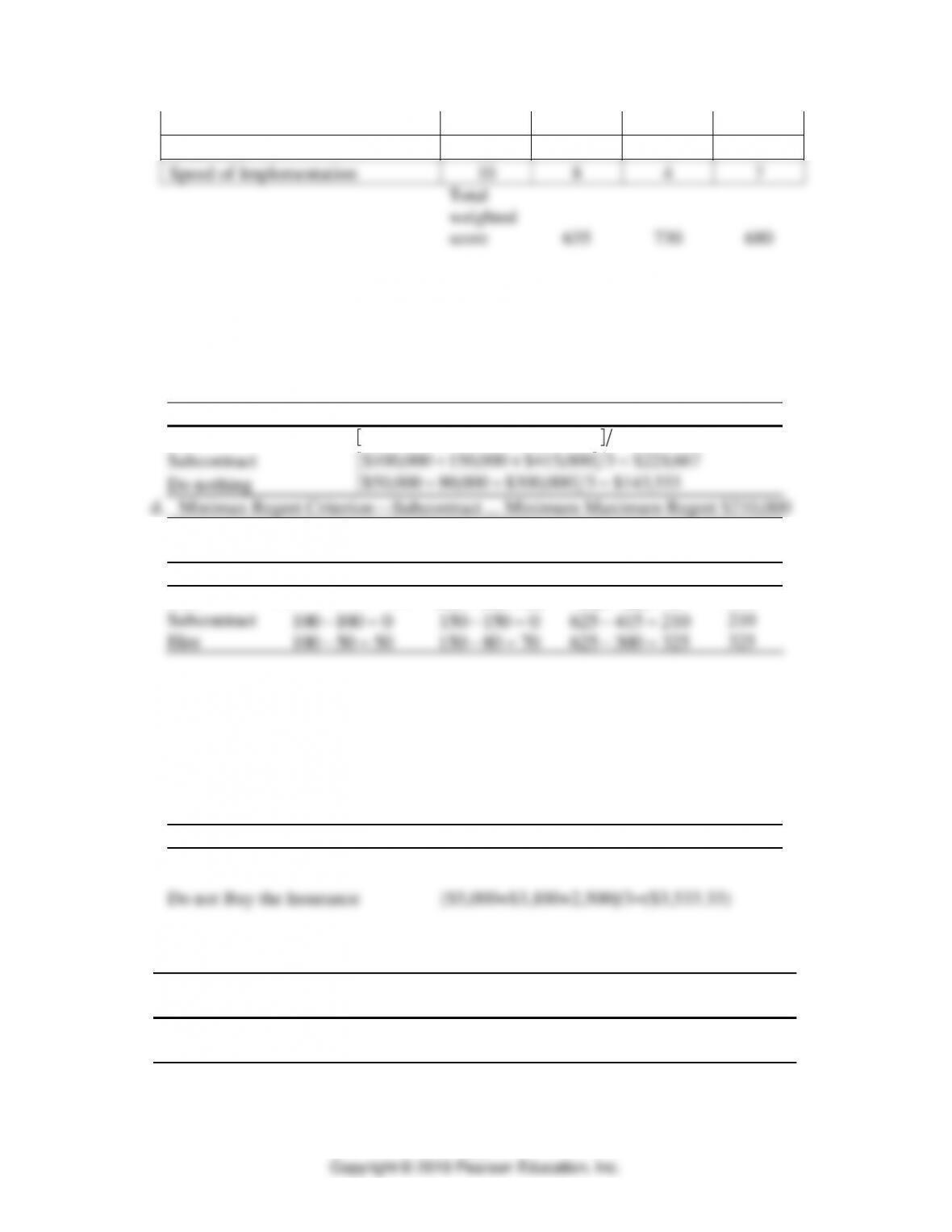
d. Minimax Regret Criterion—Subcontract … Minimum Maximum Regret $210,000
Regrets ($000)
Demand for Home Improvements
Alternative
Low
Moderate
High
Maximum
Hire
100 250 350− − =
( )
150 100 50− =
625 625 0− =
350
Subcontract
100 100 0− =
150 150 0− =
625 415 210− =
210
Hire
100 50 50− =
150 80 70− =
625 300 325− =
325
17. Robert Ragsdale
Note that this payoff table represents costs – so values closer to zero are preferred.
a. Maximin Criterion—Best Decision: Buy the Insurance … Payoff: ($2,900.00)
b. Maximax Criterion—Best Decision: Do not Buy the Insurance … Payoff: ($2,500.00)
c. Laplace Criterion—Best Decision: Buy the Insurance … Payoff: ($2,900.00)
Alternative
Weighted Payoff
Buy the Insurance
[$2,900+$2,900+$2,900]/3=($2,900)
Do not Buy the Insurance
[$5,000+$3,100+2,500]/3=($3,533.33)
d. Minimax Regret Criterion—Buy … Minimum Maximum Regret ($400)
Regrets ($000)
Demand for Home Improvements
Alternative
Computer is
Stolen
Computer
Breaks
Computer neither
is Stolen or Breaks
Maximum
Buy
2,900-2,900 =
0
2,900-2,900=
0
2,500-2,900=
-400
-400
Decision Making
A-10
Do not Buy
2,900-5,000=
-2100
2,900-3,100=
-200
2,500-2,500=
0
-2,100
18. Offshore Chemicals
The decision tree would have just one decision node with two branches (“build” and “do
not build”). The “build” alternative is followed by an event node: “Facility works” (0.40)
and “Facility fails” (0.60).
Decision Node 1
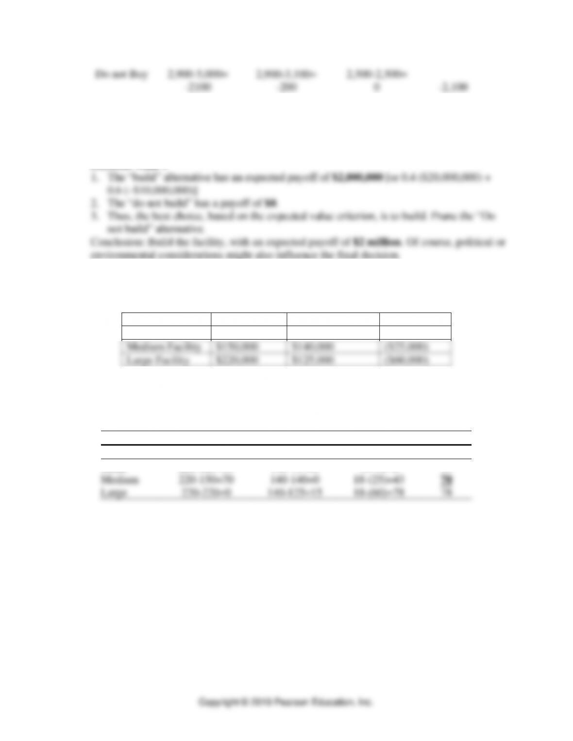
19. Small, medium, or large facility. First, develop a payoff table:
Decision
High Demand
Average Demand
Low Demand
Small Facility
$125,000
$75,000
$18,000
Medium Facility
$150,000
$140,000
($25,000)
Large Facility
$220,000
$125,000
($60,000)
a. Maximin Criterion—Best Decision: Small Facility
b. Maximax Criterion—Best Decision: Large Facility
b. Minimax Regret Criterion—Best Decision: Medium Facility
Regrets ($000)
Alternative
High
Average
Low
Maximum
Small
220-125=95
140-75=65
18-18=0
95
Medium
220-150=70
140-140=0
18-(25)=43
70
Large
220-220=0
140-125=15
18-(60)=78
78
Decision Making ⚫ SUPPLEMENT A ⚫
A-11
Decision Trees
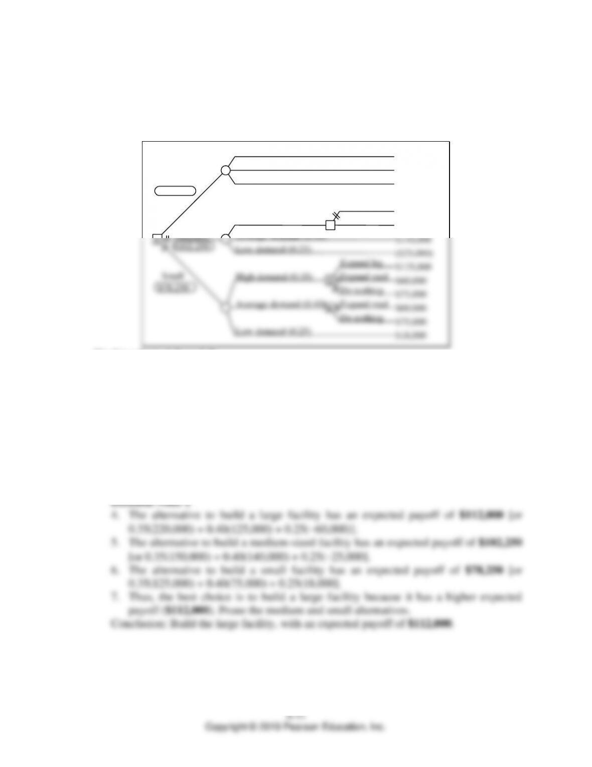
20. Small, medium, or large facility (continuation of Problem 19).
Decision Tree
Do nothing
Expand lrg
fac
Average demand (0.40)
High demand (0.35)
Low demand (0.25)
$60,000
$60,000
$18,000
3
$125,000
Do nothing
Expand lrg
fac
$112,000
Average demand (0.40)
High demand (0.35)
Low demand (0.25)
$220,000
$125,000
($60,000)
1
Large
$78,250
Small
Average demand (0.40)
High demand (0.35)
Low demand (0.25)
$150,000
$140,000
($25,000)
2
$145,000
$102,250
Medium
Expand med
ac
$75,000
Do nothing
4
$75,000
Expand med
Working from right to left:
Decision Node 2
1. The best choice is to do nothing ($150,000), which becomes the expected payoff for
Decision Node 2. Prune the “Expand to large” alternative.
Decision Node 3
2. The best choice is the “Expand to large” alternative ($125,000), which becomes the
expected payoff for Decision Node 3. Prune the “Expand to medium” and “Do
nothing” alternatives.
Decision Node 4
3. The best choice is to do nothing ($75,000), which becomes the expected payoff for
Decision Node 4. Prune the “Expand to medium” alternative.
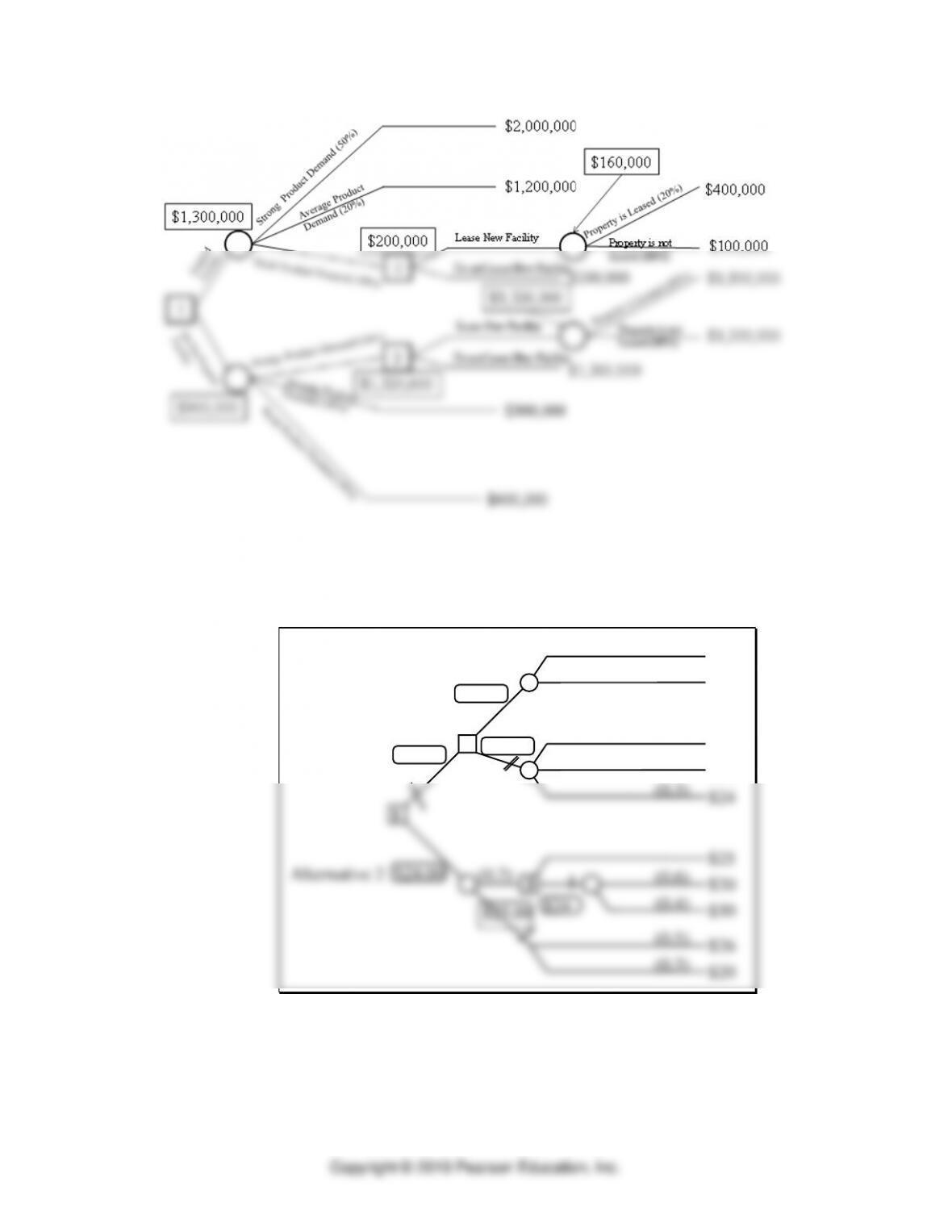
21. Pearl Automotive Dealers
As seen in the decision tree below, the best decision is to “Expand Facility” and if “Weak
Product Demand” occurs, do not attempt to lease the new expansion to an outside firm.
Decision Making
A-12
22. Decision Tree
(0.6)
(0.4)
$20
$30
$25
(0.5)
(0.5)
$15
$30
(0.3)
(0.4)
(0.3)
$20
$18
$24
1
Alternative 1
Alternative 2
$22.50
$24.00
2
$22.50
3
(0.2)
$20.60
$24
(0.5)
(0.3)
$26
$20
$25.00
Work from right to left. Here we begin with Decision Node 2, although Decision Node 3
would be an equally good starting point. The key concept is that we cannot begin analysis
of Decision Node 1 until we know the expected payoffs for Decision Nodes 2 and 3.
Decision Making ⚫ SUPPLEMENT A ⚫
A-13
Decision Node 2
1. Its first alternative (in the upper right portion of the tree) leads to an event node with an
expected payoff of $22.50 [or 0.5(15) + 0.5(30)].
Decision Node 3
4. Its second alternative leads to an event node has an expected payoff of $24 [or 0.6(20)
Decision Node 1
6. The second alternative leads to an event node has an expected payoff of $24 [or 0.2(25)
+ 0.5(26)+ 0.3(20)].
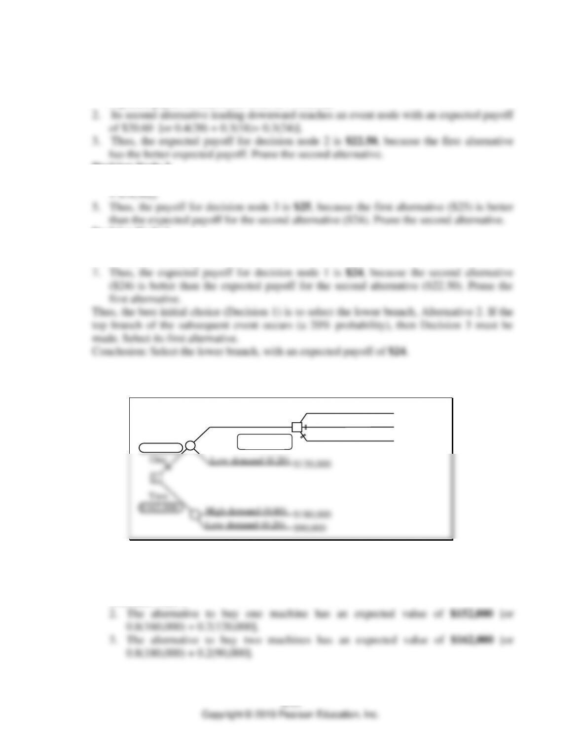
23. One machine or two.
a. Decision Tree
High demand (0.80)
Low demand (0.20)
$180,000
$90,000
$152,000
High demand (0.80)
Do nothing
Subcontract
Buy second
$160,000
$120,000
$140,000
1
One
2
Low demand (0.20)
$120,000
$162,000
Two
$160,000
b. Working from right to left:
Decision Node 2
1. The best choice is to subcontact ($160,000), which becomes the expected payoff for
Decision Node 2. Prune the “Do nothing” and Buy second” alternatives.
Decision Node 1
Decision Making
A-14
4. Thus, the best choice is to buy two machines because it has a higher expected payoff
($162,000 versus $152,000). Prune the one machine alternative.
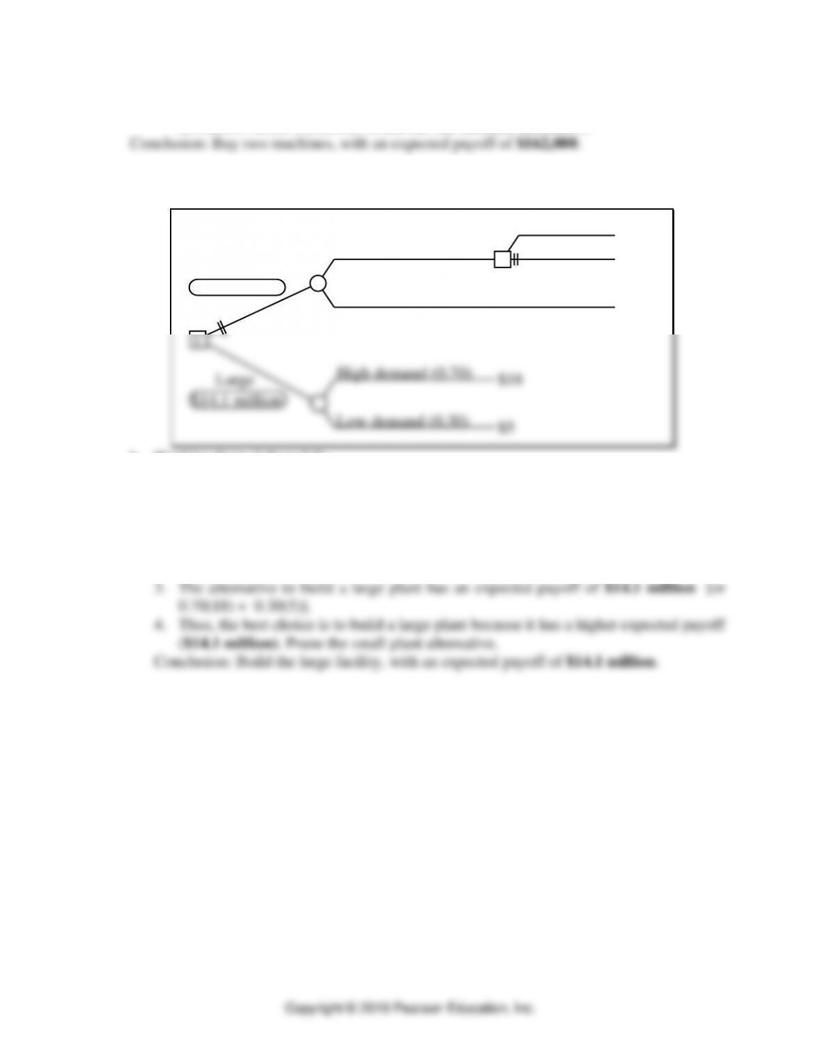
24. Small or large plant.
a. Decision Tree (payoffs are in millions of dollars)
High demand (0.70)
Low demand (0.30)
Do nothing
Expand
1
$14.1 million
Large
High demand (0.70)
Low demand (0.30)
$10
$8
2
$14
$5
$18
$12.2 million
Small
b. Working from right to left:
Decision Node 2
1. The best choice is the “Expand” alternative ($14), which becomes the expected
payoff for Decision Node 2. Prune the “Do nothing” alternative.
Decision Node 1
2. The alternative to build a small plant has an expected payoff of $12.2 million [or
0.70(14) + 0.30(8)].