• PART 2 • Managing Customer Demand
Copyright © 2019 Pearson Education, Inc.
9-18
Continuous Review (
Q
) system
Periodic Review (
P
) System
z =
1.88
Time Between Reviews (P)
2.00
Weeks
Enter manually
Safety Stock
266
Standard Deviation of Demand
d
During Protection Interval
200
Reorder Point
2266
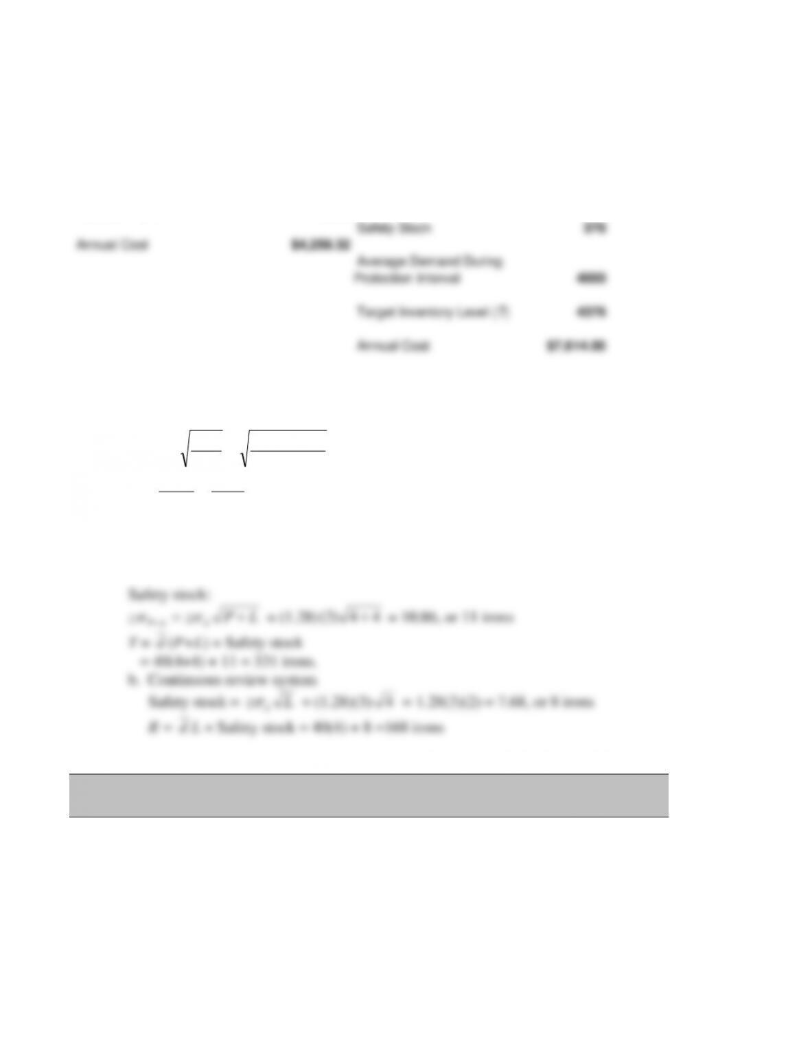
Safety Stock
376
Annual Cost
$4,258.32
Average Demand During
Protection Interval
4000
Target Inventory Level (T)
4376
Annual Cost
$7,614.00
32. Golf specialty wholesaler
a. Periodic Review System
EOQ DS
H
= = ( )( ) =
2 2 2000 40
517888.
or 179 1-irons
PEOQ
D
= = = =
179
2000 00895 4475. . years
or 4.0 weeks
When cycle-service level is 90%, z = 1.28.
Weekly demand is (2,000 units/yr)/(50 wk/yr) = 40 units/wk
L = 4 weeks
MyLab Operations Management ADVANCED PROBLEMS
1. Office Supply Shop
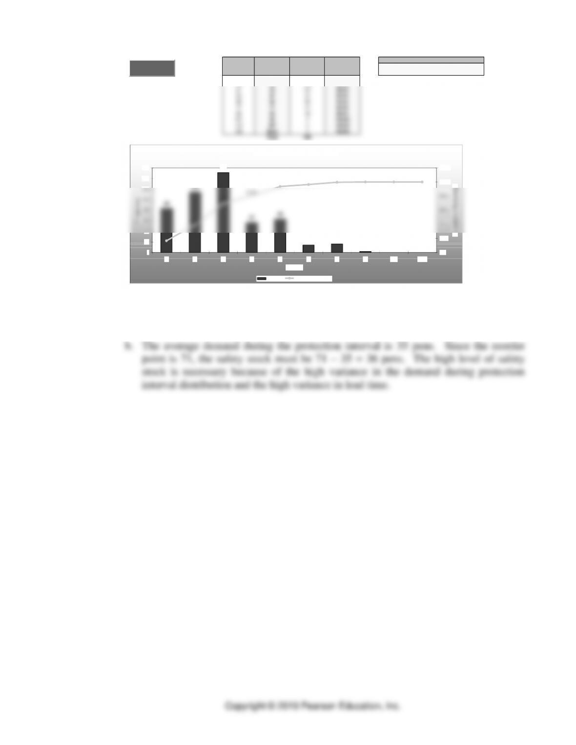
The screen shot below is taken from OM Explorer Solver – Demand During Protection
Interval Simulator. It shows the results of 500 trials.
Inventory Management • CHAPTER 9 •
9-19
17
11 83 16.6%
29
23 114 39.4%
41
35 151 69.6%
53
47 57 81.0%
65
59 63 93.6%
77
71 14 96.4%
89
83 16 99.6%
101
95 2100.0%
113
107 0100.0%
125
More 0100.0%
Total 500
Average Demand During Protection Interval
35
Demand During Protection Interval Distribution
Cumulative
Percentage
Frequency
Demand
Bin
Upper Bound
Demand During Protection Interval
83
114
151
57
63
14
16
2
0
0
16.6%
39.4%
69.6%
81.0%
93.6%
96.4%
99.6%
100.0%
100.0%
100.0%
0
20
40
60
80
100
120
140
160
11 23 35 47 59 71 83 95 107 More
Demand
Frequency
0%
20%
40%
60%
80%
100%
120%
Cumulative Percentage
Frequency Cumulative Percentage
Back to Inputs
a. Given the simulation, the value of R must yield a service level that meets or exceeds
the desired value of 95%. That value of R is 71 pens, which will yield a cycle
service level of 96.4%.
• PART 2 • Managing Customer Demand
9-20
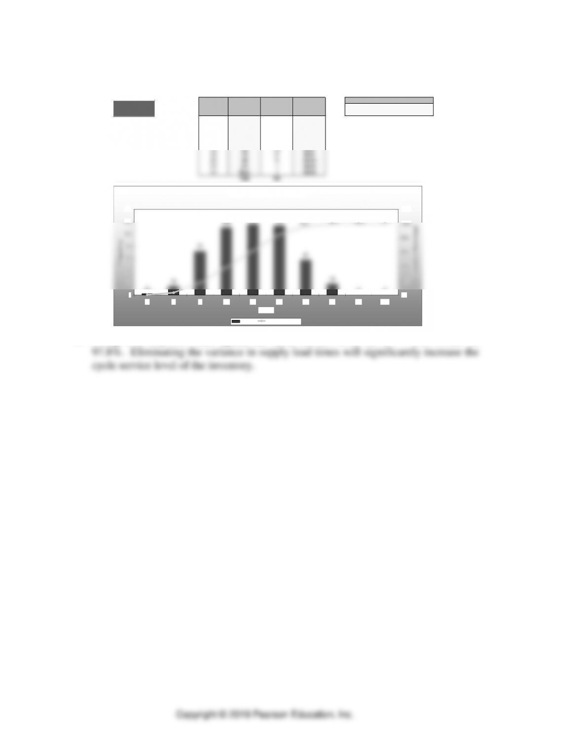
2. Grocery store.
a. The target level (T) should be 150 tubes of Happy Breath Toothpaste. This result
comes from OM Explorer Solver – Demand During Protection Interval Simulator.
60
50 20.4%
80
70 14 3.2%
100
90 71 17.4%
120
110 110 39.4%
140
130 115 62.4%
160
150 113 85.0%
180
170 57 96.4%
200
190 18 100.0%
220
210 0100.0%
240
More 0100.0%
Total 500
Average Demand During Protection Interval
132
Demand During Protection Interval Distribution
Cumulative
Percentage
Frequency
Demand
Bin
Upper Bound
Demand During Protection Interval
2
14
71
110
115
113
57
18
0
0
0.4%
3.2%
17.4%
39.4%
62.4%
85.0%
96.4%
100.0%
100.0%
100.0%
0
20
40
60
80
100
120
140
50 70 90 110 130 150 170 190 210 More
Demand
Frequency
0%
20%
40%
60%
80%
100%
120%
Cumulative Percentage
Frequency Cumulative Percentage
Back to Inputs
b. Using OM Explorer once again, the cycle-service level for T = 150 would be
Inventory Management • CHAPTER 9 •
9-21
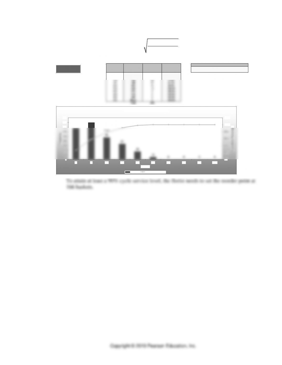
3. Floral shop
a. The EOQ for the continuous review system would be as follows.
2(2550)($30) 391
$1
Q==
The demand during protection interval distribution is shown below.
76
58 135 27.0%
112
94 159 58.8%
148
130 95 77.8%
184
166 67 91.2%
220
202 34 98.0%
256
238 10 100.0%
292
274 0100.0%
328
310 0100.0%
364
346 0100.0%
400
More 0100.0%
Total 500
Average Demand During Protection Interval
109
Demand During Protection Interval Distribution
Cumulative
Percentage
Frequency
Demand
Bin
Upper Bound
Demand During Protection Interval
135
159
95
67
34
10
0
0
0
0
27.0%
58.8%
77.8%
91.2%
98.0%
100.0%
100.0%
100.0%
100.0%
100.0%
0
20
40
60
80
100
120
140
160
180
58 94 130 166 202 238 274 310 346 More
Demand
Frequency
0%
20%
40%
60%
80%
100%
120%
Cumulative Percentage
Frequency Cumulative Percentage
Back to Inputs
• PART 2 • Managing Customer Demand
9-22
b. As the output from OM Explorer Solver – Q-System Simulator shows, the average
cost per day is $274.74.
Probability of Weekly Demand Probability of Lead Time
Probabilty of
Demand
Lower Range
Probability
Demand
(Units)
Probabilty
of Lead
Time
Lower
Range
Probability
Lead Time
(Periods)
0.40 0.00 40 0.30 0.00 1
Holding Cost ($/unit/period)
1.0$
0.30 0.40 50 0.40 0.30 2 Order Cost ($/order) 30$
0.15 0.70 60 0.20 0.70 3 Stockout Cost ($/unit) 10$
0.10 0.85 70 0.10 0.90 4
0.05 0.95 80 0.00 1.00 5 Order Size 391
1.00 1.00 Reorder Point 166
Beginning Inventory 300
Random Numbers Simulation of 50 Weeks
RN I
Demand
RN II Lead
Time
Week
Beginning
Inventory
Simulated
Demand
Ending
Inventory
Stockout
Units
Place
Order?
Simulated
Lead Time
Days to
Receive
Order
Holding
Cost
Ordering
Cost
Stockout
Cost
Total Cost
0.6586 0.8794 1 300 50 250 0No – – 275$ –$ –$ 275$
0.4101 0.2609 2 250 50 200 0No – – 225$ –$ –$ 225$
0.8676 0.5330 3 200 70 130 0 Yes 2 2 165$ 30$ –$ 195$
0.2831 0.8584 4 130 40 90 0No – 1 110$ –$ –$ 110$
0.4569 0.8724 5 481 50 431 0No – 0 456$ –$ –$ 456$
0.8689 0.9560 6 431 70 361 0No – – 396$ –$ –$ 396$
0.1591 0.2470 7 361 40 321 0No – – 341$ –$ –$ 341$
0.9864 0.9519 8 321 80 241 0No – – 281$ –$ –$ 281$
0.4978 0.8590 9 241 50 191 0No – – 216$ –$ –$ 216$
0.0223 0.7551 10 191 40 151 0 Yes 3 3 171$ 30$ –$ 201$
0.5906 0.2691 11 151 50 101 0No – 2 126$ –$ –$ 126$
0.8835 0.4734 12 101 70 31 0No – 1 66$ –$ –$ 66$
0.1373 0.4465 13 422 40 382 0No – 0 402$ –$ –$ 402$
0.0001 0.4061 14 382 40 342 0No – – 362$ –$ –$ 362$
0.7819 0.4404 15 342 60 282 0No – – 312$ –$ –$ 312$
0.9917 0.8927 16 282 80 202 0No – – 242$ –$ –$ 242$
0.5232 0.2572 17 202 50 152 0 Yes 1 1 177$ 30$ –$ 207$
0.7593 0.2128 18 543 60 483 0No – 0 513$ –$ –$ 513$
0.3090 0.8100 19 483 40 443 0No – – 463$ –$ –$ 463$
0.5006 0.6821 20 443 50 393 0No – – 418$ –$ –$ 418$
0.4173 0.5249 21 393 50 343 0No – – 368$ –$ –$ 368$
0.8148 0.4963 22 343 60 283 0No – – 313$ –$ –$ 313$
0.2962 0.2767 23 283 40 243 0No – – 263$ –$ –$ 263$
0.3003 0.1054 24 243 40 203 0No – – 223$ –$ –$ 223$
0.3560 0.7946 25 203 40 163 0 Yes 3 3 183$ 30$ –$ 213$
0.9473 0.9374 26 163 70 93 0No – 2 128$ –$ –$ 128$
0.7621 0.0953 27 93 60 33 0No – 1 63$ –$ –$ 63$
0.4240 0.2803 28 424 50 374 0No – 0 399$ –$ –$ 399$
0.9240 0.2087 29 374 70 304 0No – – 339$ –$ –$ 339$
0.3494 0.8918 30 304 40 264 0No – – 284$ –$ –$ 284$
0.9098 0.0755 31 264 70 194 0No – – 229$ –$ –$ 229$
0.0235 0.3544 32 194 40 154 0 Yes 2 2 174$ 30$ –$ 204$
0.2316 0.1659 33 154 40 114 0No – 1 134$ –$ –$ 134$
0.6310 0.8530 34 505 50 455 0No – 0 480$ –$ –$ 480$
0.8768 0.9013 35 455 70 385 0No – – 420$ –$ –$ 420$
0.8892 0.4419 36 385 70 315 0No – – 350$ –$ –$ 350$
0.4683 0.6197 37 315 50 265 0No – – 290$ –$ –$ 290$
0.3062 0.4341 38 265 40 225 0No – – 245$ –$ –$ 245$
0.3298 0.9087 39 225 40 185 0No – – 205$ –$ –$ 205$
0.1754 0.7790 40 185 40 145 0 Yes 3 3 165$ 30$ –$ 195$
0.2214 0.3099 41 145 40 105 0No – 2 125$ –$ –$ 125$
0.8985 0.4848 42 105 70 35 0No – 1 70$ –$ –$ 70$
0.8108 0.2892 43 426 60 366 0No – 0 396$ –$ –$ 396$
0.7581 0.4780 44 366 60 306 0No – – 336$ –$ –$ 336$
0.7205 0.4660 45 306 60 246 0No – – 276$ –$ –$ 276$
0.1673 0.4669 46 246 40 206 0No – – 226$ –$ –$ 226$
0.7142 0.3310 47 206 60 146 0 Yes 2 2 176$ 30$ –$ 206$
0.8320 0.0554 48 146 60 86 0No – 1 116$ –$ –$ 116$
0.9648 0.1822 49 477 80 397 0No – 0 437$ –$ –$ 437$
0.5548 0.1393 50 397 50 347 0No – – 372$ –$ –$ 372$
Inventory Management • CHAPTER 9 •
9-23
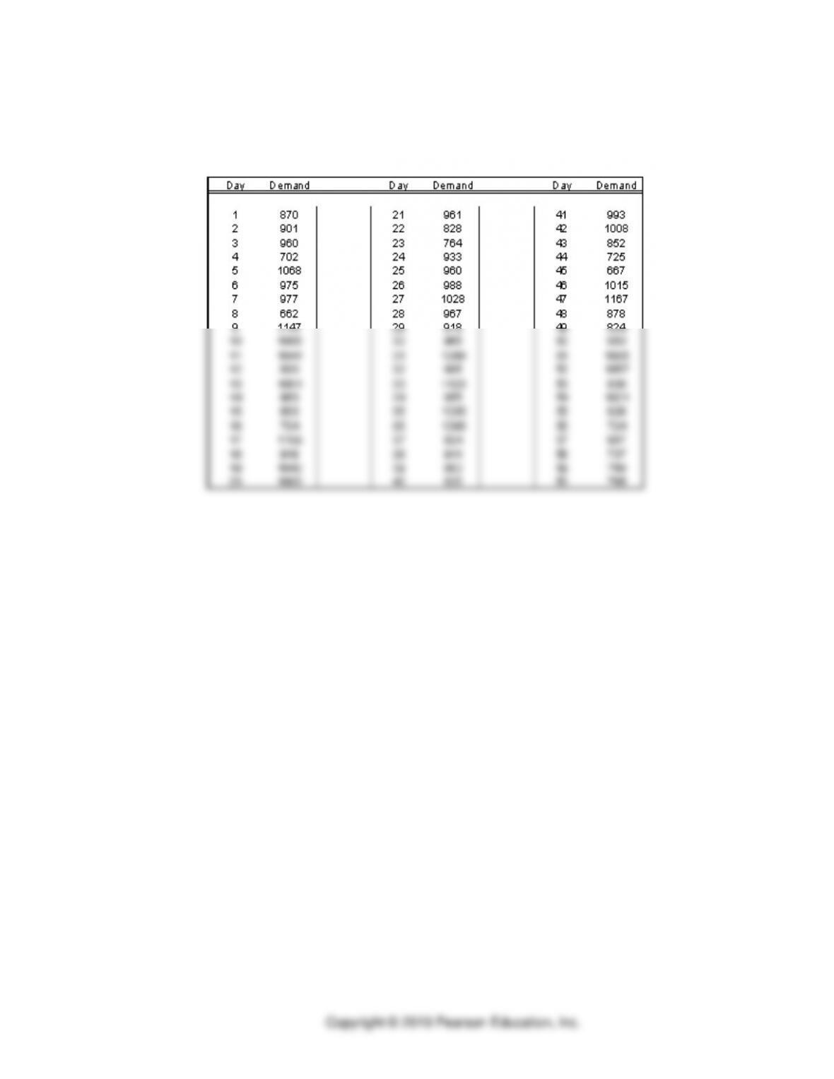
EXPERIENTIAL LEARNING: SWIFT ELECTRONIC SUPPLY, INC.
This in-class exercise allows students to test an inventory system of their design against a
new demand set. On the day of the simulation, students should come with sufficient copies
of Table 1.
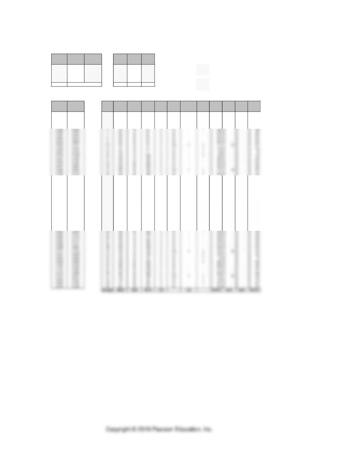
TABLE 1 1 2 . 6 | Simulation Evaluation Sheet
Day
1
2
3
4
5
6
7
8
9
10
Beginning inventory position
Number ordered
Daily demand
Day-ending inventory
Ordering costs ($200 per order)
Holding costs ($0.05 per piece per day)
Shortage costs ($2 per piece)
Total cost for day
Cumulative cost from last day
Cumulative costs to date
It is best to precede the simulation with a brief overview of the simulation process and the
calculation of costs. The instructor may decide to require students to bring a computer to
class and use a spreadsheet of their design to accomplish the tasks embodied in Table 1.
Once everyone understands the simulation procedure, the instructor uses the “actual”
demands in TN1, one at a time, and proceeding at a pace such that students have a chance to
decide whether or not to order that period, how much to order, and calculate relevant costs.
The instructor can stop at any point, using TN2 to benchmark students’ results against any of
the four provided systems in this manual. A good idea is to stop at the halfway point in the
simulation and ask students what their total costs are. The variance is often quite high. The
• PART 2 • Managing Customer Demand
9-24
TN4 through TN6 show the application of the provided systems for the demand data in
TN1. TN7 shows the results from WW system. In all of our reported results, inventory levels
at the start of the day are used to make inventory decisions. This is consistent with the daily
purchasing routine at Swift.
Economic Order Quantity (EOQ) System
Under this system, students order the EOQ each and every review period, which using the
case data would be 3 days, without any forecasts of future demand or consideration of
demand variability. TN4 shows the performance of this system. Students may elect to use
varying review periods. If so, their results will differ from TN4.
Q-system
This system assumes that inventory levels are checked on a daily basis and compared to a
“Reorder Point (RP).” If actual inventory level goes below the RP, an order of EOQ is
placed; if above, no order will be placed. In the provided results, the RP is calculated by
adding safety stock to average demand during the two-day lead time. The safety stock is
designed to meet the 95 percent cycle service level. TN5 shows the results of the Q-system.
P-system
The inventory level is reviewed every three days, which is determined by dividing EOQ
by average demand. The target inventory level is composed of two parts: “average demand
during the protection interval,” which is the review period plus the lead time, and the “safety
stock.” Every review period (three days in the provided results), an order is placed to bring
the inventory position up to the target inventory level. TN6 shows the performance of the P–
system.
Wager-Whitin (WW) System
The WW system is based on dynamic programming and assumes all demands are known
with certainty. Consequently, it provides an absolute lower bound on the solution found by
the students. The WW system assumes that stockouts are to be avoided. It is interesting to
show the difference in total costs between the WW solution and another system because it
demonstrates the cost of uncertainty. The solution using the WW system is shown in TN7.
Also note that the lot sizes are shown in the day in which they must arrive. Actual release
dates would be two days earlier. This implies that the first order for 1733 would have been
placed in day 0, one day before the actual start of the simulation.
Inventory Management • CHAPTER 9 •
9-25
TN 1. Actual Demand Data for Simulation
• PART 2 • Managing Customer Demand
9-26
TN 2. Total Costs for Four Systems
Day Demand EOQ System Q-System P-System WW Solution
1870 241.50$ 241.50$ 241.50$ 41.50$
2901 383.50$ 383.50$ 383.50$ 324.60$
3960 471.70$ 671.70$ 548.95$ 359.70$
4702 724.80$ 724.80$ 879.30$ 359.70$
51068 736.80$ 860.70$ 956.25$ 690.40$
6975 824.25$ 1,147.85$ 1,109.05$ 772.35$
7977 1,062.85$ 1,186.15$ 1,413.00$ 805.45$
8662 1,068.35$ 1,327.55$ 1,483.85$ 805.45$
91147 1,152.70$ 1,611.60$ 1,648.35$ 1,059.70$
10 1085 1,382.80$ 1,641.40$ 1,958.60$ 1,059.70$
11 1041 2,260.80$ 1,755.35$ 2,016.80$ 1,354.25$
12 890 2,352.50$ 2,024.80$ 2,175.20$ 1,404.30$
13 1001 2,594.15$ 2,044.20$ 2,483.55$ 1,404.30$
14 960 2,848.15$ 2,151.80$ 2,543.90$ 1,687.15$
15 863 2,941.20$ 2,416.25$ 2,707.70$ 1,726.85$
16 794 3,194.55$ 2,441.00$ 3,031.80$ 1,726.85$
17 1109 3,278.55$ 2,746.50$ 3,100.45$ 2,026.25$
18 948 3,367.35$ 2,804.60$ 3,252.55$ 2,078.25$
19 1040 3,604.15$ 2,946.90$ 3,552.65$ 2,078.25$
20 1008 4,148.15$ 3,238.80$ 3,602.35$ 2,367.70$
21 961 4,236.30$ 3,282.65$ 3,758.85$ 2,409.10$
22 828 4,483.05$ 3,421.30$ 4,073.95$ 2,409.10$
23 764 4,491.60$ 3,721.75$ 4,150.85$ 2,703.75$
24 933 4,589.70$ 3,775.55$ 4,320.95$ 2,751.75$
25 960 4,839.80$ 3,917.55$ 4,643.05$ 2,751.75$
35 1035 7,341.00$ 5,454.45$ 6,271.15$ 4,092.00$
36 1085 7,422.95$ 5,589.85$ 6,420.10$ 4,133.20$
37 824 7,663.70$ 5,884.05$ 6,727.85$ 4,133.20$
38 941 7,915.70$ 5,931.20$ 6,788.55$ 4,418.75$
39 883 8,007.75$ 6,070.40$ 6,952.30$ 4,460.15$
40 828 8,258.40$ 6,368.20$ 7,274.65$ 4,460.15$
41 993 8,259.40$ 6,416.35$ 7,347.35$ 4,753.15$
42 1008 8,346.20$ 6,550.30$ 7,502.25$ 4,795.75$
43 852 8,590.40$ 6,841.65$ 7,814.55$ 4,795.75$
44 725 8,598.35$ 6,896.75$ 7,890.60$ 5,079.85$
45 667 8,709.15$ 7,054.70$ 8,075.95$ 5,130.60$
Inventory Management • CHAPTER 9 •
9-27
TN 3. Cost Structure and System Parameters
In-case information EOQ System
Cost of DRAM/piece 10.00$ Average time between orders 3
Ordering cost/lot (S) 200.00$ Order Amount 2724
Stockout cost/piece per day 2.00$ Review time in EOQ system 3
Holding Cost (% of Cost of DRAM per day) 0.50%
Beginning balance 1700
The cycle inventory service level 95%
Q system
Lead tme (Days) 2
Average demand during lead time 1854
Data referred Safety stock 294
Z value at 95% confidence interval 1.645 Reorder Point for Q system 2148
Average Demand/day 927
Standard Deviation 126
Holding Cost/day 0.05$
P system
EOQ 2724 Average demand during the protection interval 4635
Safety stock 464
Review Period 3
Targeted Inventory Level 5099
• PART 2 • Managing Customer Demand
9-28
TN 4. EOQ System
Day Demand
Order
quantity
Beginning
Inventory
Ending
Inventory with
Back orders
Actual Ending
Inventory
Holding
Cost
Stockout Cost Order Cost
Daily total
Cost
Accumulative
Costs from Last
Day
Accumulative
Cost to Date
1870 2724 1700 830 830 41.50$ –$ 200.00$ 241.50$ –$ 241.50$
2901 830 -71 0 –$ 142.00$ –$ 142.00$ 241.50$ 383.50$
3960 2724 1764 1764 88.20$ –$ –$ 88.20$ 383.50$ 471.70$
4702 2724 1764 1062 1062 53.10$ –$ 200.00$ 253.10$ 471.70$ 724.80$
51068 1062 -6 0 –$ 12.00$ –$ 12.00$ 724.80$ 736.80$
6975 2724 1749 1749 87.45$ –$ –$ 87.45$ 736.80$ 824.25$
7977 2724 1749 772 772 38.60$ –$ 200.00$ 238.60$ 824.25$ 1,062.85$
20 1008 736 -272 0 –$ 544.00$ –$ 544.00$ 3,604.15$ 4,148.15$
21 961 2724 1763 1763 88.15$ –$ –$ 88.15$ 4,148.15$ 4,236.30$
22 828 2724 1763 935 935 46.75$ –$ 200.00$ 246.75$ 4,236.30$ 4,483.05$
35 1035 746 -289 0 –$ 578.00$ –$ 578.00$ 6,763.00$ 7,341.00$
36 1085 2724 1639 1639 81.95$ –$ –$ 81.95$ 7,341.00$ 7,422.95$
37 824 2724 1639 815 815 40.75$ –$ 200.00$ 240.75$ 7,422.95$ 7,663.70$
38 941 815 -126 0 –$ 252.00$ –$ 252.00$ 7,663.70$ 7,915.70$
39 883 2724 1841 1841 92.05$ –$ –$ 92.05$ 7,915.70$ 8,007.75$
40 828 2724 1841 1013 1013 50.65$ –$ 200.00$ 250.65$ 8,007.75$ 8,258.40$
41 993 1013 20 20 1.00$ –$ –$ 1.00$ 8,258.40$ 8,259.40$
42 1008 2744 1736 1736 86.80$ –$ –$ 86.80$ 8,259.40$ 8,346.20$
43 852 2724 1736 884 884 44.20$ –$ 200.00$ 244.20$ 8,346.20$ 8,590.40$
44 725 884 159 159 7.95$ –$ –$ 7.95$ 8,590.40$ 8,598.35$
45 667 2883 2216 2216 110.80$ –$ –$ 110.80$ 8,598.35$ 8,709.15$
46 1015 2724 2216 1201 1201 60.05$ –$ 200.00$ 260.05$ 8,709.15$ 8,969.20$
47 1167 1201 34 34 1.70$ –$ –$ 1.70$ 8,969.20$ 8,970.90$
48 878 2758 1880 1880 94.00$ –$ –$ 94.00$ 8,970.90$ 9,064.90$
49 824 2724 1880 1056 1056 52.80$ –$ 200.00$ 252.80$ 9,064.90$ 9,317.70$
50 863 1056 193 193 9.65$ –$ –$ 9.65$ 9,317.70$ 9,327.35$
51 1085 2917 1832 1832 91.60$ –$ –$ 91.60$ 9,327.35$ 9,418.95$
52 1067 2724 1832 765 765 38.25$ –$ 200.00$ 238.25$ 9,418.95$ 9,657.20$
53 930 765 -165 0 –$ 330.00$ –$ 330.00$ 9,657.20$ 9,987.20$
54 1021 2724 1703 1703 85.15$ –$ –$ 85.15$ 9,987.20$ 10,072.35$
55 828 2724 1703 875 875 43.75$ –$ 200.00$ 243.75$ 10,072.35$ 10,316.10$
Inventory Management • CHAPTER 9 •
9-29
TN 5. Q-System
Day
Beginning
Inventory
Demand
Ending
Inventory
with Back
Orders
Actual
Ending
Inventory
Inventory
Position
Order
Quantity
Holding Cost Stockout Cost
Ordering Cost
Daily Total
Cost
Accumulative
Costs from Last
Day
Accumulative
Cost to Date
11700 870 830 830 830 2724 41.50$ –$ 200.00$ 241.50$ –$ 241.50$
2830 901 -71 0 2724 0 –$ 142.00$ –$ 142.00$ 241.50$ 383.50$
32724 960 1764 1764 1764 2724 88.20$ –$ 200.00$ 288.20$ 383.50$ 671.70$
41764 702 1062 1062 3786 0 53.10$ –$ –$ 53.10$ 671.70$ 724.80$
53786 1068 2718 2718 2718 0 135.90$ –$ –$ 135.90$ 724.80$ 860.70$
62718 975 1743 1743 1743 2724 87.15$ –$ 200.00$ 287.15$ 860.70$ 1,147.85$
71743 977 766 766 3490 0 38.30$ –$ –$ 38.30$ 1,147.85$ 1,186.15$
83490 662 2828 2828 2828 0 141.40$ –$ –$ 141.40$ 1,186.15$ 1,327.55$
92828 1147 1681 1681 1681 2724 84.05$ –$ 200.00$ 284.05$ 1,327.55$ 1,611.60$
10 1681 1085 596 596 3320 0 29.80$ –$ –$ 29.80$ 1,611.60$ 1,641.40$
11 3320 1041 2279 2279 2279 0 113.95$ –$ –$ 113.95$ 1,641.40$ 1,755.35$
12 2279 890 1389 1389 1389 2724 69.45$ –$ 200.00$ 269.45$ 1,755.35$ 2,024.80$
13 1389 1001 388 388 3112 0 19.40$ –$ –$ 19.40$ 2,024.80$ 2,044.20$
14 3112 960 2152 2152 2152 0 107.60$ –$ –$ 107.60$ 2,044.20$ 2,151.80$
15 2152 863 1289 1289 1289 2724 64.45$ –$ 200.00$ 264.45$ 2,151.80$ 2,416.25$
16 1289 794 495 495 3219 0 24.75$ –$ –$ 24.75$ 2,416.25$ 2,441.00$
17 3219 1109 2110 2110 2110 2724 105.50$ –$ 200.00$ 305.50$ 2,441.00$ 2,746.50$
18 2110 948 1162 1162 3886 0 58.10$ –$ –$ 58.10$ 2,746.50$ 2,804.60$
19 3886 1040 2846 2846 2846 0 142.30$ –$ –$ 142.30$ 2,804.60$ 2,946.90$
20 2846 1008 1838 1838 1838 2724 91.90$ –$ 200.00$ 291.90$ 2,946.90$ 3,238.80$
21 1838 961 877 877 3601 0 43.85$ –$ –$ 43.85$ 3,238.80$ 3,282.65$
38 1884 941 943 943 3667 0 47.15$ –$ –$ 47.15$ 5,884.05$ 5,931.20$
39 3667 883 2784 2784 2784 0 139.20$ –$ –$ 139.20$ 5,931.20$ 6,070.40$
40 2784 828 1956 1956 1956 2724 97.80$ –$ 200.00$ 297.80$ 6,070.40$ 6,368.20$
41 1956 993 963 963 3687 0 48.15$ –$ –$ 48.15$ 6,368.20$ 6,416.35$
42 3687 1008 2679 2679 2679 0 133.95$ –$ –$ 133.95$ 6,416.35$ 6,550.30$
43 2679 852 1827 1827 1827 2724 91.35$ –$ 200.00$ 291.35$ 6,550.30$ 6,841.65$
44 1827 725 1102 1102 3826 0 55.10$ –$ –$ 55.10$ 6,841.65$ 6,896.75$
45 3826 667 3159 3159 3159 0 157.95$ –$ –$ 157.95$ 6,896.75$ 7,054.70$
46 3159 1015 2144 2144 2144 2724 107.20$ –$ 200.00$ 307.20$ 7,054.70$ 7,361.90$
58 2666 737 1929 1929 1929 2724 96.45$ –$ 200.00$ 296.45$ 8,958.15$ 9,254.60$
59 1929 750 1179 1179 3903 0 58.95$ –$ –$ 58.95$ 9,254.60$ 9,313.55$
60 3903 765 3138 3138 3138 0 156.90$ –$ –$ 156.90$ 9,313.55$ 9,470.45$
Average 1709.48 2662.88 953.40 85.47 2.37 70.00 157.84
Reorder Point for Q System
2148
Order Quantity 2724
• PART 2 • Managing Customer Demand
9-30
TN 6. P-System
Day
Beginning
Inventory
Demand
Ending
Inventory
with Back
orders
Actual Ending
Inventory
Inventory
Position
Order
quantity
Holding Cost
Stockout
Cost
Ordering
Cost
Daily total
Cost
Accumulative
Costs from Last
Day
Accumulative
Cost to Date
11700 870 830 830 830 4269 41.50$ –$ 200.00$ 241.50$ –$ 241.50$
2830 901 -71 0 4269 –$ 142.00$ –$ 142.00$ 241.50$ 383.50$
34269 960 3309 3309 3309 165.45$ –$ –$ 165.45$ 383.50$ 548.95$
43309 702 2607 2607 2607 2492 130.35$ –$ 200.00$ 330.35$ 548.95$ 879.30$
52607 1068 1539 1539 4031 76.95$ –$ –$ 76.95$ 879.30$ 956.25$
64031 975 3056 3056 3056 152.80$ –$ –$ 152.80$ 956.25$ 1,109.05$
73056 977 2079 2079 2079 3020 103.95$ –$ 200.00$ 303.95$ 1,109.05$ 1,413.00$
82079 662 1417 1417 4437 70.85$ –$ –$ 70.85$ 1,413.00$ 1,483.85$
94437 1147 3290 3290 3290 164.50$ –$ –$ 164.50$ 1,483.85$ 1,648.35$
10 3290 1085 2205 2205 2205 2894 110.25$ –$ 200.00$ 310.25$ 1,648.35$ 1,958.60$
11 2205 1041 1164 1164 4058 58.20$ –$ –$ 58.20$ 1,958.60$ 2,016.80$
12 4058 890 3168 3168 3168 158.40$ –$ –$ 158.40$ 2,016.80$ 2,175.20$
13 3168 1001 2167 2167 2167 2932 108.35$ –$ 200.00$ 308.35$ 2,175.20$ 2,483.55$
14 2167 960 1207 1207 4139 60.35$ –$ –$ 60.35$ 2,483.55$ 2,543.90$
15 4139 863 3276 3276 3276 163.80$ –$ –$ 163.80$ 2,543.90$ 2,707.70$
16 3276 794 2482 2482 2482 2617 124.10$ –$ 200.00$ 324.10$ 2,707.70$ 3,031.80$
17 2482 1109 1373 1373 3990 68.65$ –$ –$ 68.65$ 3,031.80$ 3,100.45$
18 3990 948 3042 3042 3042 152.10$ –$ –$ 152.10$ 3,100.45$ 3,252.55$
19 3042 1040 2002 2002 2002 3097 100.10$ –$ 200.00$ 300.10$ 3,252.55$ 3,552.65$
20 2002 1008 994 994 4091 49.70$ –$ –$ 49.70$ 3,552.65$ 3,602.35$
21 4091 961 3130 3130 3130 156.50$ –$ –$ 156.50$ 3,602.35$ 3,758.85$
22 3130 828 2302 2302 2302 2797 115.10$ –$ 200.00$ 315.10$ 3,758.85$ 4,073.95$
23 2302 764 1538 1538 4335 76.90$ –$ –$ 76.90$ 4,073.95$ 4,150.85$
39 4158 883 3275 3275 3275 163.75$ –$ –$ 163.75$ 6,788.55$ 6,952.30$
40 3275 828 2447 2447 2447 2652 122.35$ –$ 200.00$ 322.35$ 6,952.30$ 7,274.65$
41 2447 993 1454 1454 4106 72.70$ –$ –$ 72.70$ 7,274.65$ 7,347.35$
42 4106 1008 3098 3098 3098 154.90$ –$ –$ 154.90$ 7,347.35$ 7,502.25$
43 3098 852 2246 2246 2246 2853 112.30$ –$ 200.00$ 312.30$ 7,502.25$ 7,814.55$
44 2246 725 1521 1521 4374 76.05$ –$ –$ 76.05$ 7,814.55$ 7,890.60$
45 4374 667 3707 3707 3707 185.35$ –$ –$ 185.35$ 7,890.60$ 8,075.95$
46 3707 1015 2692 2692 2692 2407 134.60$ –$ 200.00$ 334.60$ 8,075.95$ 8,410.55$
47 2692 1167 1525 1525 3932 76.25$ –$ –$ 76.25$ 8,410.55$ 8,486.80$
55 3148 828 2320 2320 2320 2779 116.00$ –$ 200.00$ 316.00$ 9,696.20$ 10,012.20$
56 2320 724 1596 1596 4375 79.80$ –$ –$ 79.80$ 10,012.20$ 10,092.00$
57 4375 987 3388 3388 3388 169.40$ –$ –$ 169.40$ 10,092.00$ 10,261.40$
58 3388 737 2651 2651 2651 2448 132.55$ –$ 200.00$ 332.55$ 10,261.40$ 10,593.95$
59 2651 750 1901 1901 4349 95.05$ –$ –$ 95.05$ 10,593.95$ 10,689.00$
60 4349 765 3584 3584 3584 179.20$ –$ –$ 179.20$ 10,689.00$ 10,868.20$
Average 2219 3196.441 2882.5 110.97$ 2.41$ 66.67$ 181.17$
Inventory Management • CHAPTER 9 •
9-31
TN 7. Wagner-Whitin (WW) Solution
Period
Demand
Lot Size
End Inventory
End Backorder
Cum. Cost
1700
1
870
0
830
0
41.5
2
901
1733
1662
0
324.6
3
960
0
702
0
359.7
4
702
0
0
0
359.7
5
1068
3682
2614
0
690.4
6
975
0
1639
0
772.35
7
977
0
662
0
805.45
8
662
0
0
0
805.45
9
1147
2232
1085
0
1059.7
10
1085
0
0
0
1059.7
11
1041
2932
1891
0
1354.25
12
890
0
1001
0
1404.3
13
1001
0
0
0
1404.3
14
960
2617
1657
0
1687.15
15
863
0
794
0
1726.85
16
794
0
0
0
1726.85
17
1109
3097
1988
0
2026.25
18
948
0
1040
0
2078.25
19
1040
0
0
0
2078.25
20
1008
2797
1789
0
2367.7
21
961
0
828
0
2409.1
22
828
0
0
0
2409.1
23
764
2657
1893
0
2703.75
24
933
0
960
0
2751.75
25
960
0
0
0
2751.75
26
988
2983
1995
0
3051.5
27
1028
0
967
0
3099.85
28
967
0
0
0
3099.85
29
918
2951
2033
0
3401.5
30
965
0
1068
0
3454.9
31
1068
0
0
0
3454.9
32
996
2974
1978
0
3753.8
33
1123
0
855
0
3796.55
34
855
0
0
0
3796.55
35
1035
2944
1909
0
4092
36
1085
0
824
0
4133.2
37
824
0
0
0
4133.2
38
941
2652
1711
0
4418.75
39
883
0
828
0
4460.149
40
828
0
0
0
4460.149
41
993
2853
1860
0
4753.149
42
1008
0
852
0
4795.75
43
852
0
0
0
4795.75
44
725
2407
1682
0
5079.85
45
667
0
1015
0
5130.6
46
1015
0
0
0
5130.6
47
1167
3732
2565
0
5458.85
48
878
0
1687
0
5543.2
49
824
0
863
0
5586.35
50
863
0
0
0
5586.35
51
1085
3082
1997
0
5886.2
52
1067
0
930
0
5932.7
53
930
0
0
0
5932.7
54
1021
2573
1552
0
6210.3
55
828
0
724
0
6246.5
56
724
0
0
0
6246.5
57
987
3239
2252
0
6559.1
58
737
0
1515
0
6634.85
59
750
0
765
0
6673.1
60
765
0
0
0
6673.1
Average
902.3
973.9
Minimum Total Cost
6673.10
• PART 2 • Managing Customer Demand
9-32
CASE: PARTS EMPORIUM
A. Synopsis
This case describes the problems facing Sue McCaskey, the new materials manager of a
wholesale distributor of auto parts. She seeks ways to cut the bloated inventories while
improving customer service. Back orders with excessive lost sales are all too frequent.
Inventories were much higher than expected when the new facility was built, even
though sales have not increased. Summary data on inventory statistics, such as
inventory turns, are not available. McCaskey decides to begin with a sample of two
products to uncover the nature of the problems—the EG151 exhaust gasket and the
DB032 drive belt.
B. Purpose
The purpose of this case is to allow the student to put together a plan, using either a
continuous review system (Q system) or a periodic review system (P system), for two
inventory SKUs. Enough information is available to determine the EOQ and R for a
continuous review system (or P and T for a periodic review system). Because stockouts
are costly relative to inventory holding costs, a 95% cycle-service level is
recommended. Inventory holding costs are 21% of the value of each item (expressed at
cost). The ordering costs ($20 for exhaust gaskets and $10 for drive belts) should not be
increased to include charges for making customer deliveries. These charges are
independent of the inventory replenishment at the warehouse and are reflected in the
pricing policy.
C. Analysis
We now find appropriate policies for a Q system, beginning with the exhaust gasket. Shown
here are the calculations of the EOQ and R, followed by a cost comparison between this
continuous review system and the one now being used. The difference is what can be
realized by a better inventory control system. Reducing lost sales due to back orders is surely
the biggest benefit.
1. EG151 Exhaust Gasket
a. New plan
Begin by estimating annual demand and the variability in the demand during the
lead time for this first item. Working with the weekly demands for the first 21
weeks of this year and assuming 52 business weeks per year, we find the EOQ
as follows:
Weekly demand average = 102 gaskets/week
Annual demand (D) = 102(52) = 5304 gaskets
Holding cost = $1.85 per gasket per year (or 0.21 0.68 $12.99)
Ordering cost = $20 per order
( )( )
EOQ 2 5,304 $20 $1.85 339==
gaskets
Copyright © 2019 Pearson Education, Inc.
b. Cost comparison
After developing their plan, students can compare its annual cost with what
would be experienced with current policies.
Cost Category
Current Plan
Proposed Plan
Ordering cost
$707
$313
Holding cost (cycle inventory)
139
314
TOTAL
$846
$627
The total of these two costs for the gasket is reduced by 26 percent (from $846 to
$627) per year. The safety stock with the proposed plan may be higher than the
current plan, if the reason for the excess back orders is that no safety stock is now
being held (inaccurate inventory records or a faulty replenishment system are other
explanations). We cannot determine the safety stock level (if any) in the current
2. DB032 Drive Belt
a. New plan
The following demand estimates are based on weeks 13 through 21. Weeks 11
and 12 are excluded from the analysis because the new product’s start-up makes
them unrepresentative. We find the EOQ as follows:
Weekly demand average = 52 belts/week
Annual demand (D) = 52(52) = 2704 belts
Holding cost $0.97 per belt per year (or 0.21 0.52 $8.89)
Ordering cost $10 per order
( )( )
EOQ 2 2,704 $10 $0.97 236==
gaskets
Turning now to R, where z remains at 1.65, we use the data in the DB032 table
to find:
Standard deviation in weekly demand (
d
) = 1.76 belts
Standard deviation in demand during lead time
05.3376.1 ==
dLT
belts
R = Average demand during the lead time + Safety stock
9-33
• PART 2 • Managing Customer Demand
9-34
= 3(52) + 1.65(3.05) = 161.03, or 161 belts
b. Cost comparison
After developing their plan, students again can compare the cost for the belts
with what would be experienced with current policies.
Cost Category
Current Plan
Proposed Plan
Ordering cost
$ 27
$115
Holding cost (cycle inventory)
485
114
TOTAL
$512
$229
With the belt, the total of these two costs is reduced by 55 percent. The safety
service level implemented with the proposed plan.
D. Recommendations
For the gasket, the recommendation is to implement a continuous review system with
Q = 339 and R = 211. For the belt, the recommendation is to implement a continuous
review system with Q = 236 and R = 161.
E. Teaching Strategy
This case can be used as a “cold–call” case or as a short case prepared in advance of the
class meeting. If used without prior student preparation, it works best as a team
assignment. Each team can have a different assignment (P or Q system, gasket or belt).
When used as a cold-call case and time is a concern, the instructor should provide the
mean and standard deviation of the weekly demand for the two products.
Begin with a general discussion of how to do the analysis and then work through the
analysis. If done with teams, give each time to follow through. After the teams develop
their policies, have them make the cost comparison. It brings back the fundamental
notions of cycle inventory and ordering costs that were introduced in this Inventory
Management chapter. The discussion at the end can broaden into other issues, such as
applying the notion of inventory levers and the use of systems other than a Q system to
control inventories.
If time permits, the instructor can have the class hand-simulate their policies, using the
actual demand data in the first 21 weeks of this year for the gaskets and the last 9 weeks
of this year for the belts. Use a form to record the simulation, either as a handout or
transparency. The starting conditions on back orders, scheduled receipts, and on-hand
inventory can be what is mentioned in the case for week 21.