Chapter
9
Inventory Management
DISCUSSION QUESTIONS
1. The short answer is that higher inventories do not provide an advantage in any of the
nine competitive priority categories. The important point is that firms must have the
“right amount” of inventory to meet their competitive priorities.
The only relevant costs considered in this chapter are ordering costs, holding costs, and
stockout costs. In the economic order quantity (EOQ) model, costs of placing
does L.
1. Low-cost operations. Costs include materials, scrap, labor, and equipment capacity
that are wasted when products are defective. When a process drifts out of control,
competitor H’s large lot sizes tend to result in large quantities of defectives. The
EOQ does not consider the cost of defectives, and erroneously assumes that setup
costs are constant. Small lots cause frequent setups, but the cost per setup decreases
• PART 2 • Managing Customer Demand
9-2
5. On-time delivery. Contrary to expectations, large inventories do not equate to on-
time delivery. It’s more like, lots of inventory equals lots of chaos. Big lots make
big scheduling problems. Big lots get dropped, mishandled, and pilfered. Most lean
companies experience dramatic improvement in on-time delivery.
In summary, a case can be made that several competitive priorities are not considered in
the EOQ model. It is sometimes difficult to place a dollar value on these competitive
advantages, but the advantages invariably go to the low-inventory, small lot-size firm.
So, if the EOQ is too large, what is the “ideal” lot size? According to the lean
philosophy, the “ideal” lot size is one.
2. The continuous review system requires the determination of two parameters: the order
quantity and the reorder point. The ordering cost for each firm will decrease, which
means that the economic order quantities will decrease. Because of this, there may be
some implications for the logistics system. Smaller, more frequent shipments could
require more costly less-than-truckload shipments. In addition, while the order
3. Organizations will never get to the point where inventories are unneeded. Inventories
provide many functions and should be managed, not eliminated. It is impossible to
Inventory Management • CHAPTER 9 •
9-3
PROBLEMS
Types of Inventory
1. A part
a. Average cycle inventory
=Q2
= =
1000 2 500 units
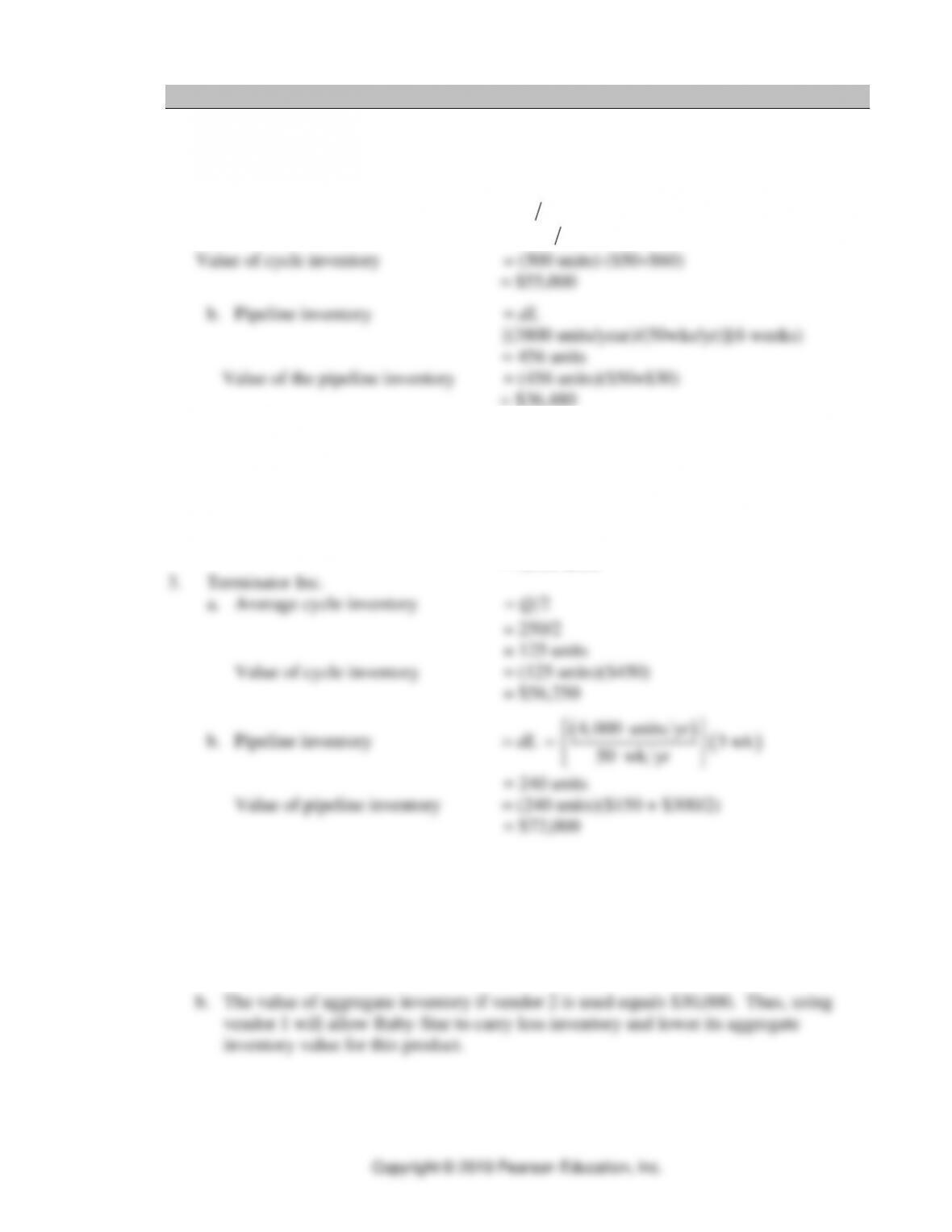
2. Prince Electronics
a. Value of each DC’s pipeline inventory
= (75 units/wk)(2 wk)($350/unit)
= $52,500
b. Total inventory = cycle + safety + pipeline
= 5[(400/2) + (2*75) + (2*75)]
= 2,500 units
Inventory Reduction Tactics
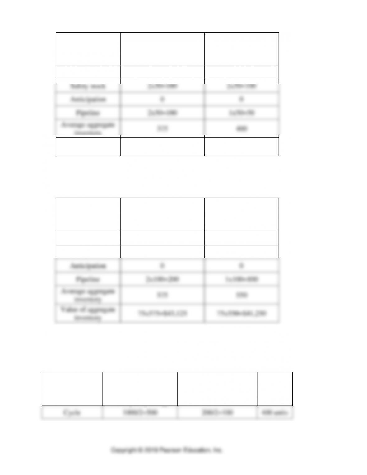
4. Ruby-Star Incorporated
a. As seen in the Table below, the value of aggregate inventory if vendor 1 is used
equals $28,125
• PART 2 • Managing Customer Demand
9-4
Type of Inventory
Calculation of aggregate
average inventory value
for vendor 1
Calculation of
aggregate average
inventory value for
vendor 2
Cycle
350/2 = 175
500/2=250
Safety stock
2×50=100
2×50=100
Anticipation
0
0
Pipeline
2×50=100
1×50=50
Average aggregate
inventory
375
400
Value of aggregate
inventory
75×375=$28,125
75×400=$30,000
c. As seen in the table below, if average weekly demand increased to 100 units per
week, the value of aggregate inventory using vendor 1 is now greater than using
vendor 2.
Type of Inventory
Calculation of aggregate
average inventory value
for vendor 1
Calculation of
aggregate average
inventory value for
vendor 2
Cycle
350/2 = 175
500/2=250
Safety stock
2×100=200
2×100=200
Anticipation
0
0
Pipeline
2×100=200
1×100=100
Average aggregate
inventory
575
550
Value of aggregate
inventory
75×575=$43,125
75×550=$41,250
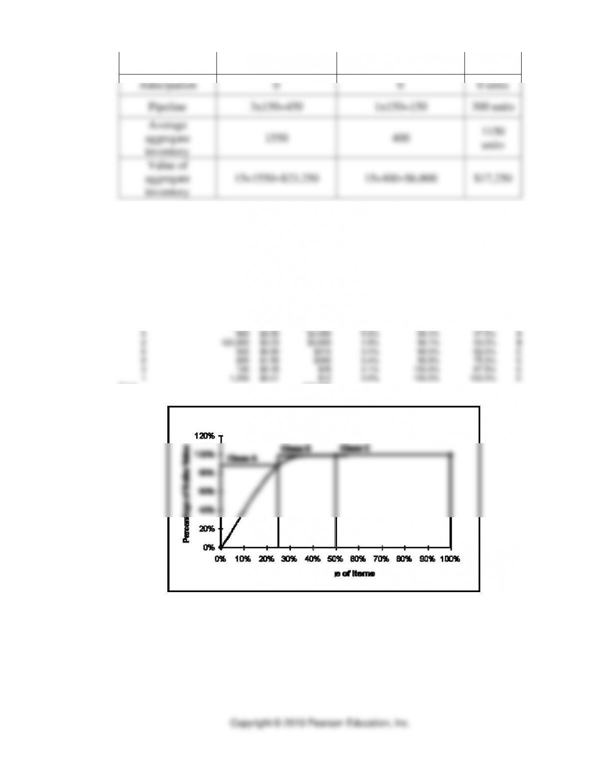
5. Haley Photocopying
The policy changes enabled by the new vendor location will allow Haley to reduce
their average inventory level by 1,150 units and their average aggregate inventory
value by $17,250 for paper.
Type of Inventory
Calculation of
aggregate average
inventory and its value
before policy change
Calculation of aggregate
average inventory and its
value after policy change
Savings
Cycle
1000/2=500
200/2=100
400 units
Inventory Management • CHAPTER 9 •
9-5
Safety stock
4×150=600
1×150=150
450 units
Anticipation
0
0
0 units
Pipeline
3×150=450
1×150=150
300 units
Average
aggregate
inventory
1550
400
1150
units
Value of
aggregate
inventory
15×1550=$23,250
15×400=$6,000
$17,250
ABC Analysis
6. Oakwood Hospital
First we rank the SKUs from top to bottom on the basis of their dollar usage. Then we
partition them into classes. The analysis was done using OM Explorer Tutor 9.2—ABC
Analysis.
Cumulative %
Cumulative %
SKU #
Description
Qty Used/Year
Value
Dollar Usage
Pct of Total
of Dollar Value
of SKUs
Class
4
44,000
$1.00
$44,000
60.0%
60.0%
12.5%
A
7
70,000
$0.30
$21,000
28.6%
88.7%
25.0%
A
5
900
$4.50
$4,050
5.5%
94.2%
37.5%
B
2
120,000
$0.03
$3,600
4.9%
99.1%
50.0%
B
6
350
$0.90
$315
0.4%
99.5%
62.5%
C
8
200
$1.50
$300
0.4%
99.9%
75.0%
C
3
100
$0.45
$45
0.1%
100.0%
87.5%
C
1
1,200
$0.01
$12
0.0%
100.0%
100.0%
C
Total
$73,322
SKUs
• PART 2 • Managing Customer Demand
9-6
The dollar usage percentages don’t exactly match the predictions of ABC analysis. For
example, Class A SKUs account for 88.7% of the total, rather than 80%. Nonetheless,
the important finding is that ABC analysis did find the “significant few.” For the items
sampled, particularly close control is needed for SKUs 4 and 7.
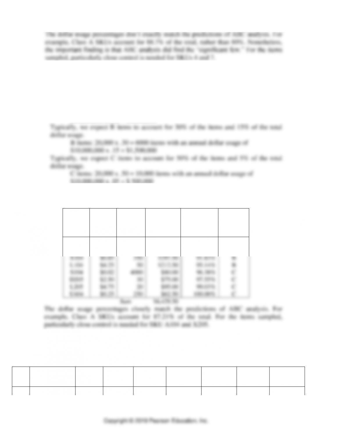
7. Southern Markets Inc.
a. Typically, we expect A items to account for 20% of the items and 80% of the
total dollar usage.
A items: 20,000 x .20 = 4000 items with an annual dollar usage of
$10,000,000 x .80 = $8,000,000
$10,000,000 x .05 = $ 500,000
b. First, we rank the SKUs from top to bottom based upon their annual dollar
usage. Then we partition them into classes. The analysis was done using
Excel.
SKU
Code
Unit
Value
Demand
(units)
Annual
Dollar
Usage
Cumulative
Percentage
of Dollar
Usage
Item
Category
A104
$2.10
2500
$5,250.00
81.65%
A
X205
$0.35
1020
$357.00
87.21%
A
X104
$0.85
350
$297.50
91.83%
B
L104
$4.25
50
$212.50
95.14%
B
S104
$0.02
4000
$80.00
96.38%
C
D205
$2.50
30
$75.00
97.55%
C
L205
$4.75
20
$95.00
99.03%
C
U404
$0.25
250
$62.50
100.00%
C
Sum
$6,429.50
The dollar usage percentages closely match the predictions of ABC analysis. For
example, Class A SKUs account for 87.21% of the total. For the items sampled,
particularly close control is needed for SKU A104 and X205.
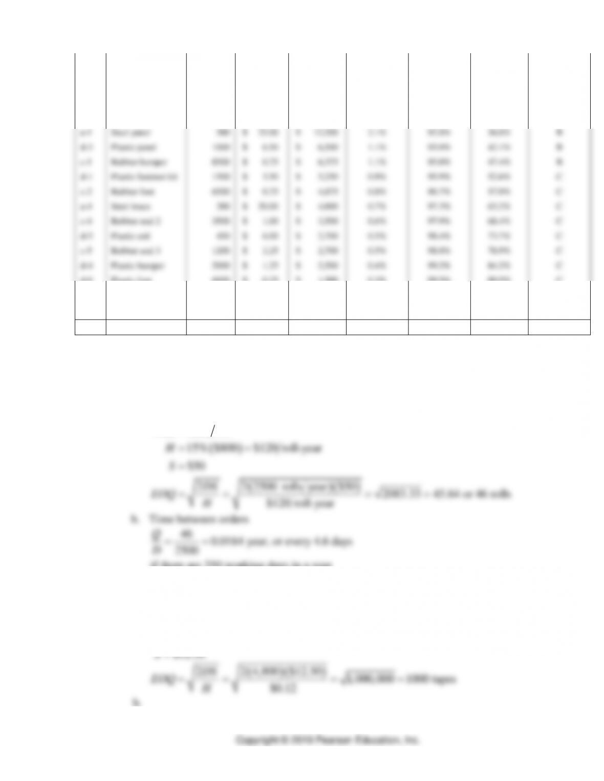
8. New Wave Shelving
The dollar usage percentages closely match the predictions of ABC analysis. Class A
SKUs account for 81.6% of the total and B SKUs account for 13.4% of the total.
SKU
#
Description
Quantity
Used Per
Year
Dollar
Value Per
Unit
Annual
Dollar
Usage
Percent
Dollar Usage
of the Total
Cumulative
percent of
Dollar Usage
Cumulative
percent of
SKU items
Classification
b-1
Copper coil
1250
$ 260.00
$ 325,000
54.2%
54.2%
5.3%
A
Inventory Management • CHAPTER 9 •
9-7
a-2
Steel bumper
750
$ 135.00
$ 101,250
16.9%
71.1%
10.5%
A
b-2
Copper panel
1250
$ 50.00
$ 62,500
10.4%
81.6%
15.8%
A
b-3
Copper brace 1
250
$ 75.00
$ 18,750
3.1%
84.7%
21.1%
B
b-4
Copper brace 2
150
$ 125.00
$ 18,750
3.1%
87.8%
26.3%
B
a-3
Steel clamp
3500
$ 5.00
$ 17,500
2.9%
90.8%
31.6%
B
a-1
Steel panel
500
$ 25.00
$ 12,500
2.1%
92.8%
36.8%
B
d-3
Plastic panel
1000
$ 6.50
$ 6,500
1.1%
93.9%
42.1%
B
c-1
Rubber bumper
8500
$ 0.75
$ 6,375
1.1%
95.0%
47.4%
B
d-1
Plastic fastener kit
1500
$ 3.50
$ 5,250
0.9%
95.9%
52.6%
C
c-2
Rubber foot
6500
$ 0.75
$ 4,875
0.8%
96.7%
57.9%
C
a-4
Steel brace
200
$ 20.00
$ 4,000
0.7%
97.3%
63.2%
C
c-4
Rubber seal 2
3500
$ 1.00
$ 3,500
0.6%
97.9%
68.4%
C
d-5
Plastic coil
450
$ 6.00
$ 2,700
0.5%
98.4%
73.7%
C
c-5
Rubber seal 3
1200
$ 2.25
$ 2,700
0.5%
98.8%
78.9%
C
d-4
Plastic bumper
2000
$ 1.25
$ 2,500
0.4%
99.2%
84.2%
C
d-6
Plastic foot
6000
$ 0.25
$ 1,500
0.3%
99.5%
89.5%
C
c-3
Rubber seal 1
1500
$ 1.00
$ 1,500
0.3%
99.7%
94.7%
C
d-2
Plastic handle
2000
$ 0.75
$ 1,500
0.3%
100.0%
100.0%
C
Sum
$ 599,150
Economic Order Quantity
9. Yellow Press, Inc.
a. Economic order quantity
( )
( )( )
2500 rolls
Price $800 roll
15% $800 $120 roll-year
$50
2 2 2500 rolls year $50 2083.33 45.64 or 46 rolls
$120 roll-year
D
H
S
DS
EOQ H
=
=
==
=
= = = =
b. Time between orders
46 0.0184 year, or every 4.6 days
2500
if there are 250 working days in a year
==
Q
D
10. Babble Inc.
a.
D = 400 tapes/month)(12 months/yr) = 4,800 tapes/year
$0.12
$12.50
H
S
=
=
( )( )
2 2 4,800 $12.50 1,000,000 1000 tapes
$0.12
DS
EOQ H
= = = =
b.
• PART 2 • Managing Customer Demand
9-8
Time between orders
1, 000 0.2083
4,800
Q
D==
years or 2.5 months
11. Dot Com
a.
( )( )
2 32,000 $10
2400 books
$4
DS
EOQ H
= = =
12. Leaky Pipe Inc.
a.
( )( )
2 30,000 $10
2775 units
$1
DS
EOQ H
= = =
Continuous Review Systems
13. Sam’s Cat Hotel
a. Economic order quantity
d
= 90/week
D = (90 bags/week)(52 weeks/yr) = 4,680
D= = =
4680 008547 444. . years weeks
b. Reorder point, R
R = demand during protection interval + safety stock
When the desired cycle-service level is 80%,
z=084.
.
Inventory Management • CHAPTER 9 •
9-9
L
ddLT
=
= 15
3
= 25.98 or 26
Safety stock = 0.84 * 26 = 21.82, or 22 bags
R= + =270 22 292
c. Initial inventory position = OH + SR – BO = 320 + 0 – 0
d. Annual holding cost Annual ordering cost
QH
2
500
227% 70
75
=( )( )
=
$11.
$789.
4,680 $54
500
$505.44
=
=
DS
Q
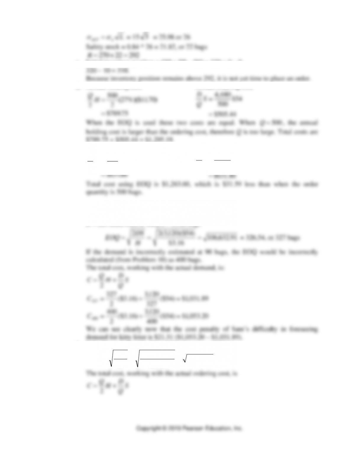
When the EOQ is used these two costs are equal. When
Q=500
, the annual
holding cost is larger than the ordering cost, therefore Q is too large. Total costs are
$789.75 + $505.44 = $1,295.19.
e. Annual holding cost Annual ordering cost
QH
2
400
227% 70
80
=( )( )
=
$11.
$631.
4,680 $54
400
$631.80
DS
Q=
=
14. Sam’s Cat Hotel, revisited
a. If the demand is only 60 bags per week, the correct EOQ is:
D = (60 units/wk)(52 wk/yr) = 3,120 bags
91.632,106
16.3$
)54)($120,3(22 === H
DS
EOQ
= 326.54, or 327 bags
If the demand is incorrectly estimated at 90 bags, the EOQ would be incorrectly
calculated (from Problem 10) as 400 bags.
The total cost, working with the actual demand, is:
2
QD
C H S
Q
=+
89.031,1$)54($
327
120,3
)16.3($
2
327
327 =+=C
20.053,1$)54($
400
120,3
)16.3($
2
400
400 =+=C
We can see clearly now that the cost penalty of Sam’s difficulty in foreseeing
demand for kitty litter is $21.31 ($1,053.20 – $1,031.89).
b. If S = $6, and
D= =60 52 3120
, the correct EOQ is:
10.848,11
16.3$
)6)($120,3(22 === H
DS
EOQ
= 108.85, or 109 bags
2
Q
• PART 2 • Managing Customer Demand
9-10
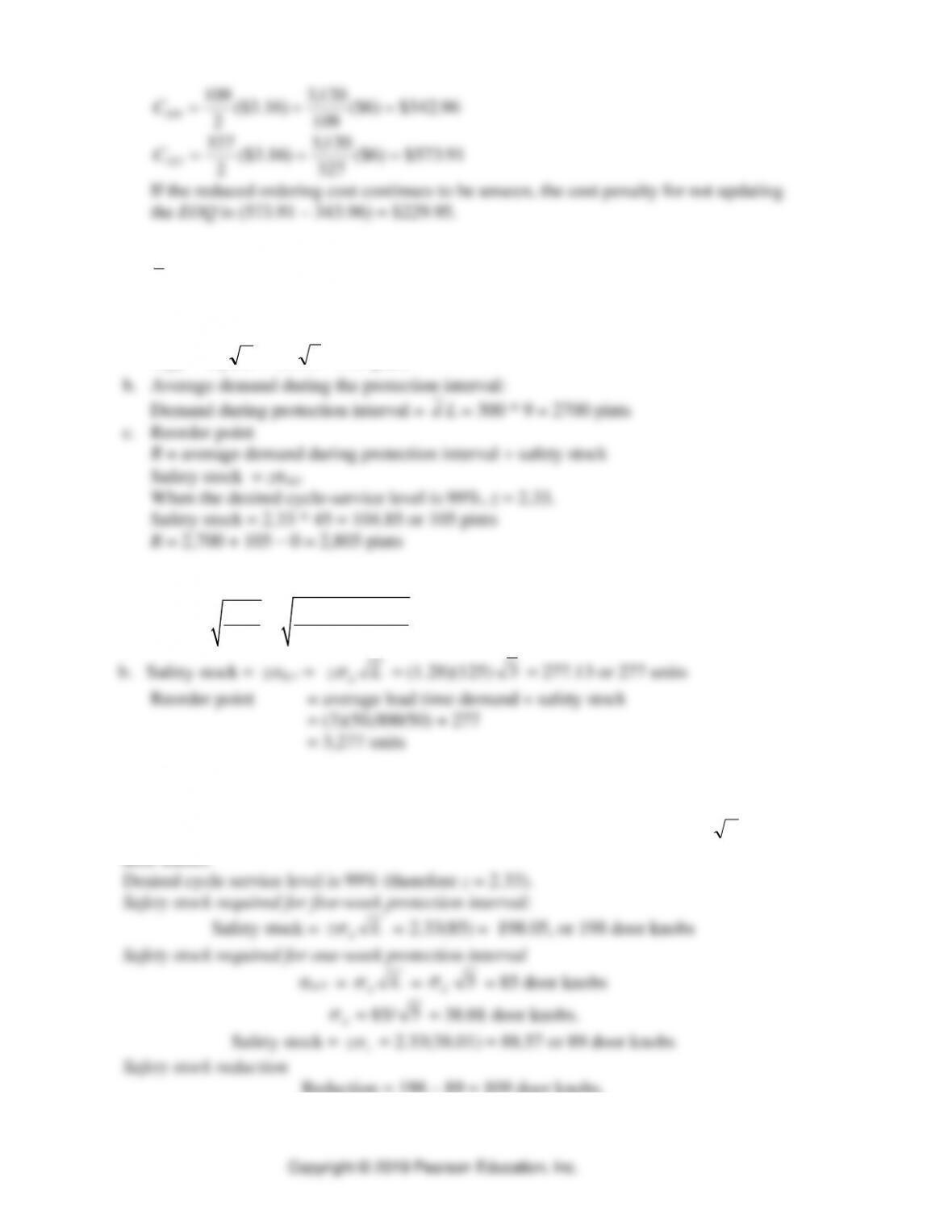
96.342$)6($
109
120,3
)16.3($
2
109
109 =+=C
91.573$)6($
327
120,3
)16.3($
2
327
327 =+=C
If the reduced ordering cost continues to be unseen, the cost penalty for not updating
the EOQ is (573.91 – 343.96) = $229.95.
15. A Q system (also known as a reorder point system)
d
= 300 pints/week
d
= 15 pints
a. Standard deviation of demand during the protection interval:
L
ddLT
=
= 15
9
= 45 pints
16. Petromax Enterprises
a.
( )( )
2 50,000 35
21,323 units
2
DS
EOQ H
= = =
3
17. A continuous review system for door knobs.
Find the safety stock reduction when lead time is reduced from five weeks to one week.
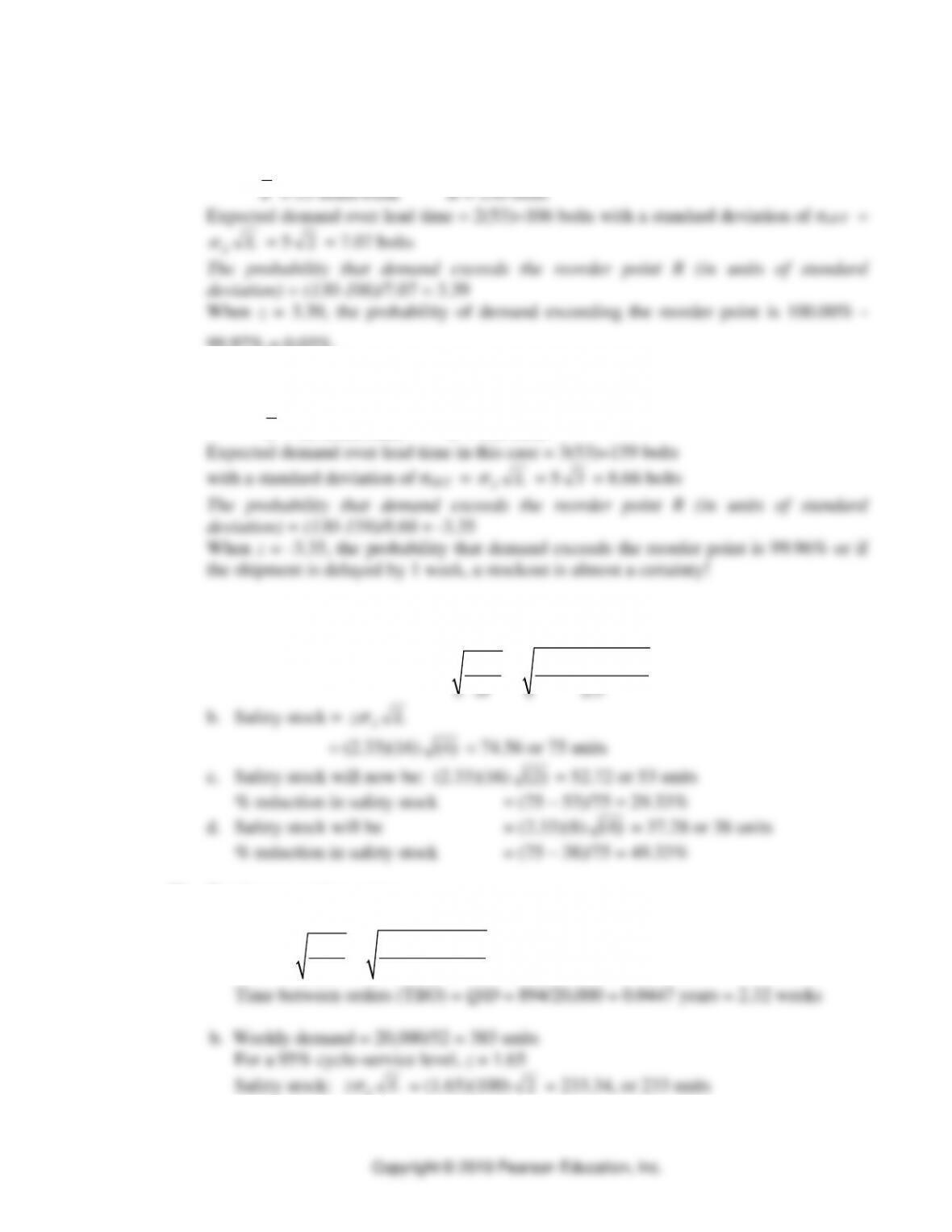
Standard deviation of demand during the (five-week) protection interval is
L
d
= 85
door knobs.
Reduction = 198 – 89 = 109 door knobs.
Inventory Management • CHAPTER 9 •
9-11
18. A two-bin system. “The two-bin system is really a Q system, with the normal level in
the second bin being the reorder point R.”
a. Find cycle-service level, given:
L = 2 weeks
d
= 5 bolts
d
99.97% = 0.03%.
b. Using the same approach as in part (a), given:
L = 3 weeks
d
= 5 bolts
d
= 53 bolts/week R = 130 bolts
19. A Successful Product
Annual Demand, D = (200)(50) = 10,000 units, H = ((0.20)(12.50)) = 2.50
a. Optimal ordering quantity
( )( )
2 10,000 50
2633 units
2.5
DS
H
= = =
20. Continuous review system.
a. Economic order quantity.
( )( )
2 2,000 40
2894.4
2
DS
EOQ H
= = =
or 894 units
• PART 2 • Managing Customer Demand
9-12
Now solve for R, as
R =
d
L + Safety stock = 385(2) + 233 = 1,003 units
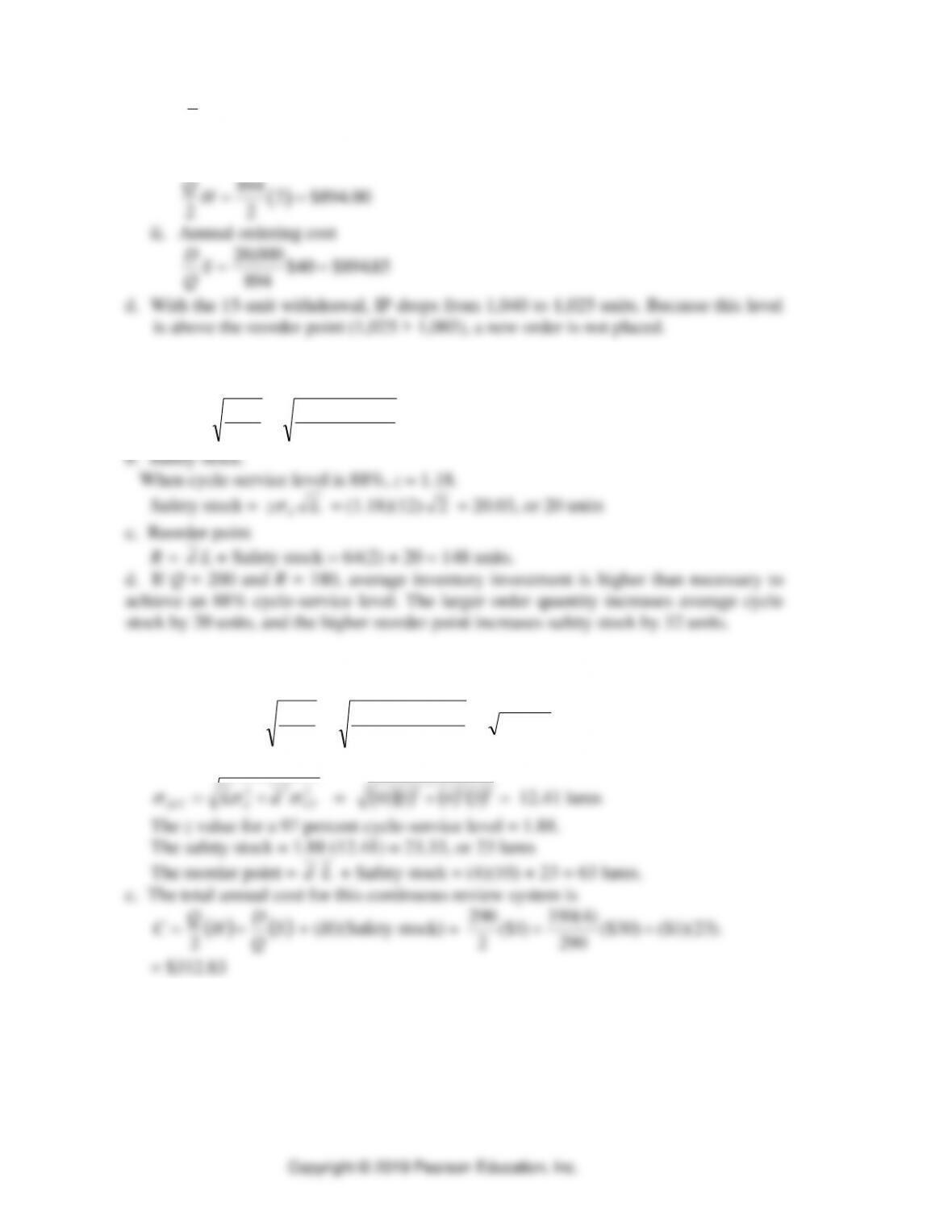
c. i. Annual holding cost of cycle inventory
( )
894 2 $894.00
22
QH==
ii. Annual ordering cost
D
QS= =
20 000
894 85
,$40 $894.
d. With the 15-unit withdrawal, IP drops from 1,040 to 1,025 units. Because this level
is above the reorder point (1,025 > 1,003), a new order is not placed.
21. Continuous review system
a. Economic order quantity
EOQ DS
H
= = ( )( )( ) =
2 2 64 52 50
13 160 units
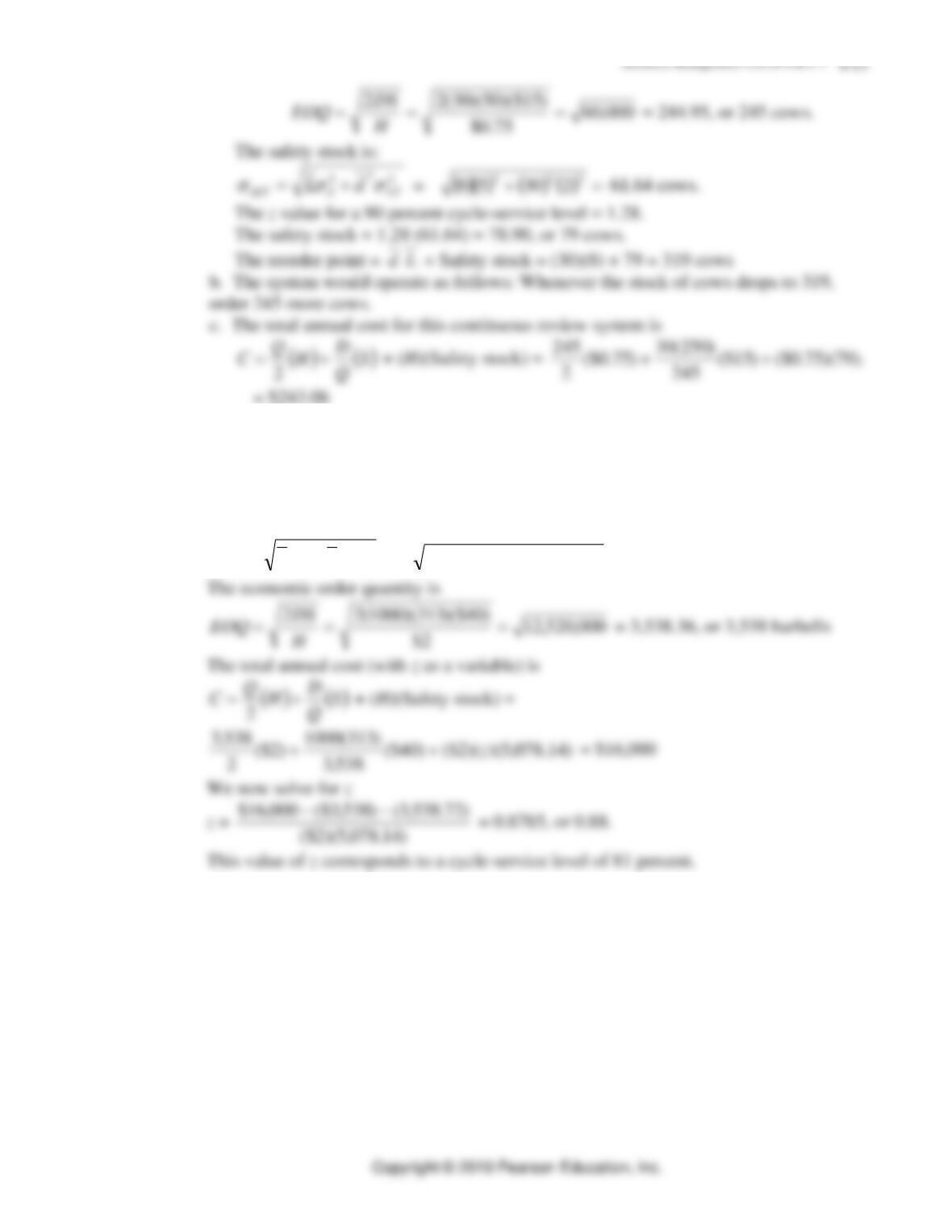
22. Osprey Sports.
a. The economic order quantity is
000,84
1$
)30)($4)(350(22 === H
DS
EOQ
= 289.83, or 290 lures.
b. The safety stock and reorder point are
2
2
2
LTddLT dL
+=
=
( )( ) ( ) ( )
=+ 222 34110
12.41 lures
The z value for a 97 percent cycle-service level = 1.88.
The safety stock = 1.88 (12.41) = 23.33, or 23 lures
The reorder point =
d
L
+ Safety stock = (4)(10) + 23 = 63 lures.
c. The total annual cost for this continuous review system is
( ) ( )
S
Q
D
H
Q
C+= 2
+ (H)(Safety stock) =
).23)(1($)30($
290
)4(350
)1($
2
290 ++
= $312.83
23. Farmer’s Wife
a. The continuous review system is specified by the fixed order quantity and the
reorder point. We will use the EOQ for the order quantity.
The order quantity is:
Copyright © 2019 Pearson Education, Inc.
24. Muscle Bound
To find the cycle-service level, we must determine the standard deviation of demand
during lead time and then use the equation for total annual cost to solve for z. We will
use the EOQ for the ordering quantity.
The standard deviation of demand during lead time is
2
2
2
LTddLT dL
+=
=
( )( ) ( ) ( )
=+ 222 5100015035
5,078.14 barbells
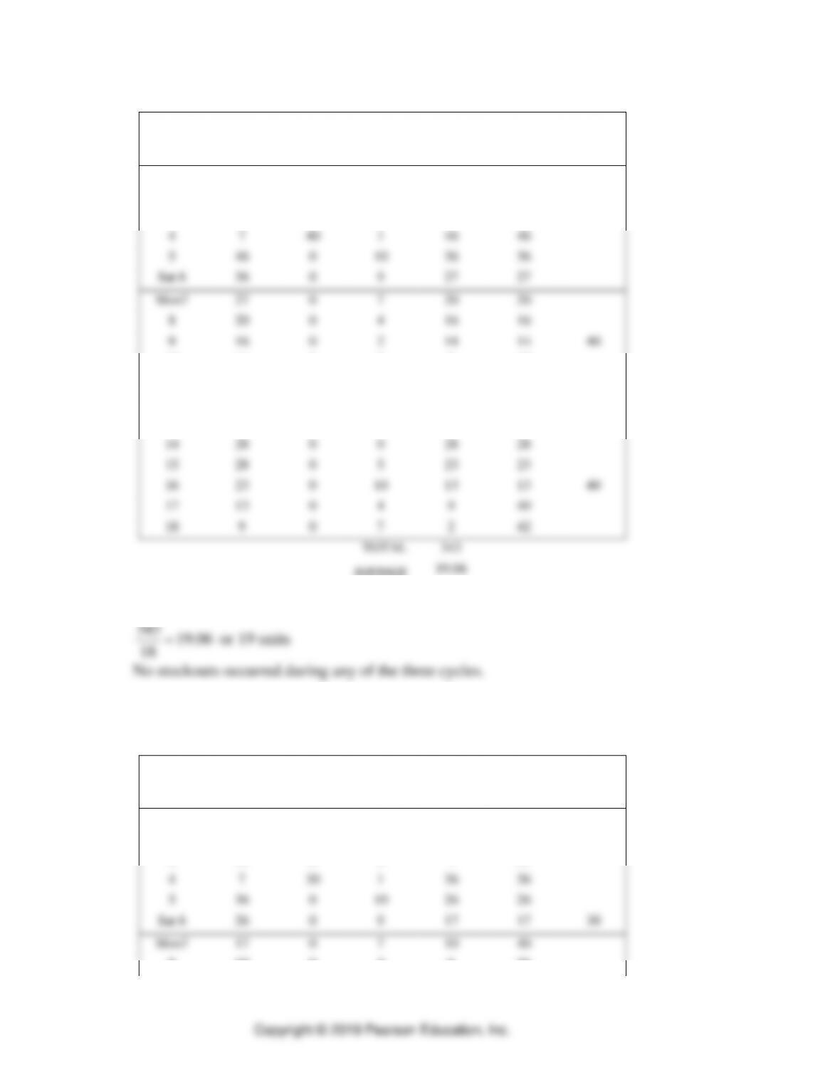
25. Georgia Lighting Center.
Using the demand data given in the problem statement, we extended text Table 9.2
below the dashed line in the following way. The beginning inventory for day 7 is the
ending inventory for day 6, which is 27 units. The demand for day 7 is 7 units, which
leaves 20 units in inventory at the end of day 7. No orders are open to the supplier;
consequently, the inventory position is 20 units. Because 20 units exceeds the reorder
point of 15 units, no new order is placed. Continuing in this manner, the inventory
position at the end of day 9 drops below the reorder point; consequently, a new order
for 40 units is placed. That order will be received three business days later, or day 12.
The complete simulation results with Q = 40 and R = 15 are:
• PART 2 • Managing Customer Demand
9-14
Day
Beginning
Inventory
Open
Orders
Received
Daily
Demand
Ending
Inventory
Inventory
Position
Amount
Ordered
1
19
0
5
14
14
40
2
14
0
3
11
51
3
11
0
4
7
47
4
7
40
1
46
46
5
46
0
10
36
36
Sat 6
36
0
9
27
27
Mon7
27
0
7
20
20
8
20
0
4
16
16
9
16
0
2
14
14
40
10
14
0
7
7
47
11
7
0
3
4
44
12
4
40
6
38
38
13
38
0
10
28
28
14
28
0
0
28
28
15
28
0
5
23
23
16
23
0
10
13
13
40
17
13
0
4
9
49
18
9
0
7
2
42
TOTAL
343
AVERAGE
19.06
a. The average ending inventory is:
343 19.06
18 =
or 19 units
No stockouts occurred during any of the three cycles.
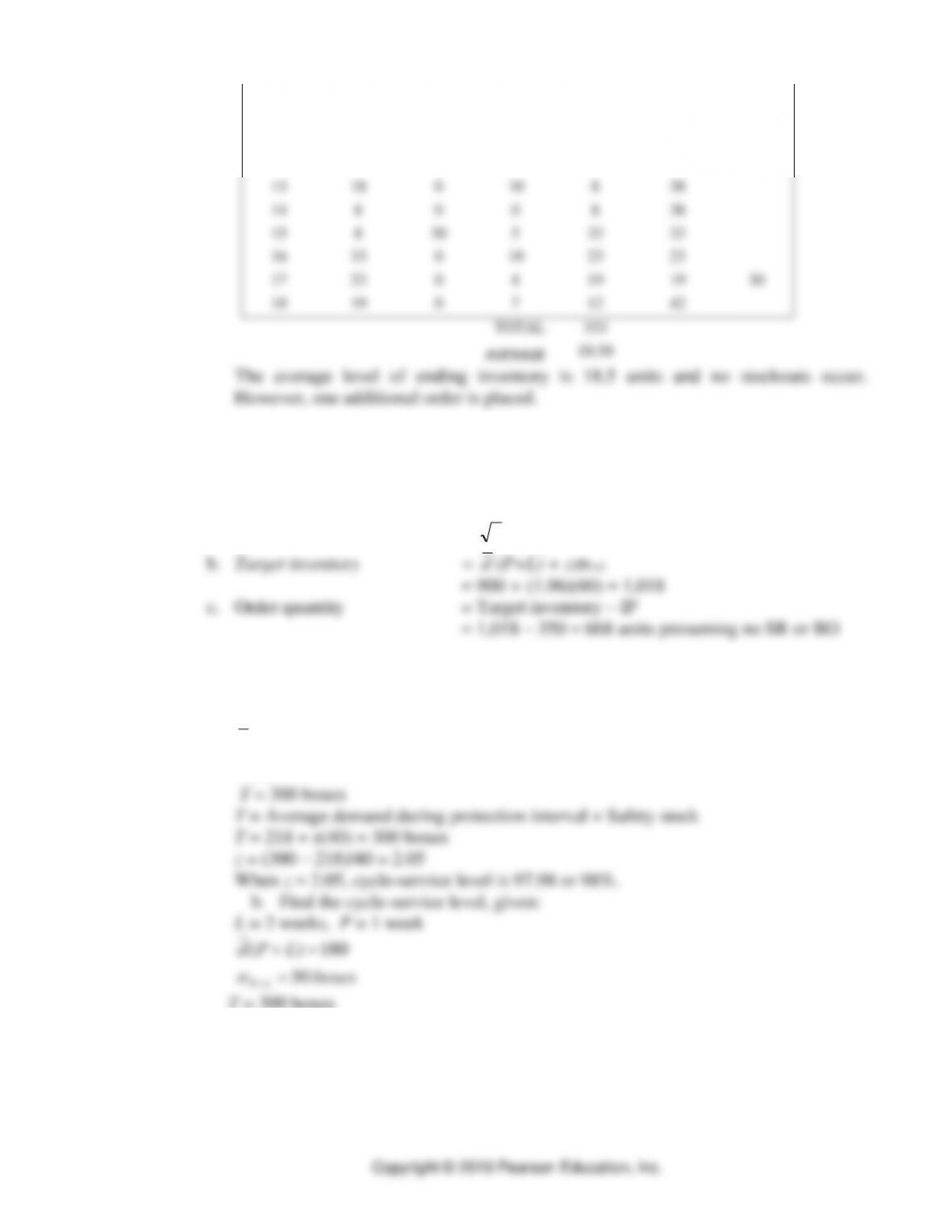
b. Assuming a Q=30, R= 20 system is used, the following simulation results:
Day
Beginning
Inventory
Open
Orders
Received
Daily
Demand
Ending
Inventory
Inventory
Position
Amount
Ordered
1
19
0
5
14
14
30
2
14
0
3
11
41
3
11
0
4
7
37
4
7
30
1
36
36
5
36
0
10
26
26
Sat 6
26
0
9
17
17
30
Mon7
17
0
7
10
40
8
10
0
4
6
36
Inventory Management • CHAPTER 9 •
9-15
9
6
30
2
34
34
10
34
0
7
27
27
11
27
0
3
24
24
12
24
0
6
18
18
30
13
18
0
10
8
38
14
8
0
0
8
38
15
8
30
5
33
33
16
33
0
10
23
23
17
23
0
4
19
19
30
18
19
0
7
12
42
TOTAL
333
AVERAGE
18.50
The average level of ending inventory is 18.5 units and no stockouts occur.
However, one additional order is placed.
Periodic Review System
26. Nationwide Auto Parts
a. Protection interval (PI) = P + L = 6 +3 = 9 weeks
Average demand during PI = 9 (100) = 900 units
Standard deviation during PI =
)20(9 •
= 60 units
27. P system (also known as a periodic review system) for weed killer.
a. Find cycle-service level, given:
L = 2 weeks, P = 1 week
( ) 218
40
PL
d P L
boxes
+
+=
=
50
PL
boxes
+
=
T = 300 boxes
T = Average demand during protection interval + Safety stock
T = 180 + z(20) = 300 boxes
z = (300 – 180)/50 = 2.40
When z = 2.40, cycle-service level is 99.18 or 99%.
• PART 2 • Managing Customer Demand
9-16
28. Sam’s Cat Hotel with a P system
a. Referring to Problem13, the EOQ is 400 bags. When the demand rate is 15 per day,
the average time between orders is (400/15) = 26.67 or about 27 days. The lead time
is 3 weeks 6 days per week = 18 days. If the review period is set equal to the
EOQ’s average time between orders (27 days), then the protection interval (P + L)
= (27 + 18) = 45 days.
29. Periodic review system
a. Economic order quantity.
2 2(15,080)(125) 1121
3
DS
EOQ units
H
= = =
b. Continuous Review System
Weekly demand = 15,080/52 = 290 units
For a 95% cycle-service level, z = 1.65
c. The periodic review system has a longer protection interval and thereby requires
more safety stock. In this case: 317-236 = 81 units
Inventory Management • CHAPTER 9 •
9-17
30. Periodic review system
a. From Problem 21, EOQ = 160
5.2
64
160EOQ === d
P
weeks
P is rounded to 3 weeks.
31. Wood County Hospital
a. D = (1000 boxes/wk)(52 wk/yr) = 52,000 boxes
H = (0.l5)($35/box)=$5.25/box
( )( )
2 52,000 $15
2545.1 or 545 boxes
$5.25
DS
EOQ H
= = =
900
545
2
900 52,000
$5.25 $15.00 $3, 229.16
2 900
545 52,000
$5.25 $15.00 $2,861.82
2 545
QD
C H S
Q
C
C
=+
= + =
= + =
The savings would be $3,229.16 – $2,861.82 = $367.34.
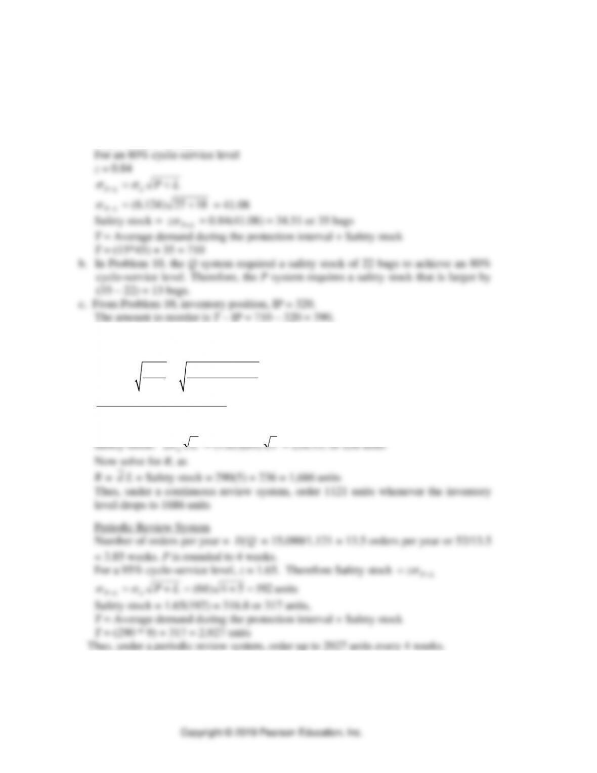
b. When the cycle-service level is 97%, z = 1.88. Therefore,
Safety stock =
Lz d
= (1.88)(100)
2
= 1.88(141.42) = 265.87, or 266 boxes
R =
d
L + Safety stock = 1000(2) + 266 = 2,266 boxes
c. In a periodic review system, find target inventory T, given:
P = 2 weeks
L = 2 weeks
Safety stock =
zP L
+
LP
dLP +=
+
22)100( +=
+LP
= 200 units.
Safety stock = 1.88(200) = 376 units
T = Average demand during the protection interval + Safety stock
T = 1000(2 + 2) + 376
T = 4,376 units
The table below is derived from OM Explorer Solver—Inventory Systems. Notice
that the total cost for the Q system is much less than that of the P system. The
reason is that the optimal value of P was not used here. The optimal value is
P=055.
weeks.