Chapter
9 Inventory Management
TEACHING TIP
Open with Ford’s Smart Inventory Management System (SIMS) and its use of big data to
ascertain what customers want, manage vehicle complexity, and distribute the “right” cars to the
“right” dealers.
Managing inventories is a process that requires information about expected demands, amounts of
inventory on hand and on order for every item stocked by the firm at all locations, and the
appropriate timing and size of the reorder quantities. This chapter focuses on the decision-
making aspects of this process.
Inventory Management
1. Inventories are important to all types of organizations and their employees.
a. Inventories affect everyday operations because they have to be counted, paid for, used in
operations, used to satisfy customers, and managed.
b. Inventories require an investment of funds.
c. Monies invested in inventory are not available for investment in other things.
2. Inventory a boon or bane?
a. Too much inventory on hand reduces profitability.
b. Too little inventory on hand damages customer confidence.
c. Inventory management involves trade-offs.
1. Inventory Tradeoffs
The flow of materials determines inventory levels. Inventory is a stock of materials used to satisfy
customer demand or to support the production of services or goods.
Use Figure 9.1 to show how inventories are created through the analogy of a water tank.
The inward flow of water represents input materials
The water level represents the amount of inventory held
The outward flow of water represents the demand for materials in inventory
Inventory level is the difference between input flow rate and the output flow rate
An inventory manager’s job is to balance the advantages and disadvantages of both small and
large inventories and find a happy medium between the two levels.
1. Pressures for small inventories
a. Inventory holding cost (the sum of the cost of capital plus the variable costs of keeping
items on hand)
b. Cost of capital (opportunity cost of investing in an asset relative to the expected return on
assets of similar risk)
c. Storage and handling costs (An inventory holding cost is incurred when a firm could use
storage space productively in some other way)
d. Taxes, insurance, and shrinkage
• Pilferage (theft of inventory by customers or employees)
• Obsolescence (inventory cannot be used or sold at full value, owing to model
changes, engineering modifications, or unexpectedly low demand)
• Deterioration (physical spoilage or damage due to rough or excessive material
handling results in lost value)
2. Pressures for large inventories
a. Customer service (speed delivery and improve the firm’s on-time delivery)
• Stockout (is an order that cannot be satisfied, resulting in loss of the sale)
• Backorder (order that cannot be filled when promised or demanded but is filled later)
TEACHING TIP
Use Managerial Practice 9.1 Inventory Management at Netflix to illustrate how inventory
management supports competing priorities such as variety and delivery speed and how process
design may reduce the need for excessive inventory investment.
b. Ordering cost (the cost of preparing a purchase order)
c. Setup cost (cost involved in changing over a machine or workspace to produce a different
item)
d. Labor and equipment utilization (inventory built during slack periods to handle extra
demand)
e. Transportation cost (inventory on hand allows more full-carload shipments to be made
and minimizes the need to expedite shipments)
f. Payments to suppliers
• Quantity discount
• Supplement C, “Special Inventory Models,” shows how to determine order
quantities.
2. Types of inventory
1. Accounting Inventories: Inventory exists in three aggregate categories that are useful for
accounting purposes.
a. Raw materials
b. Work-in-process
c. Finished goods
d. An important distinction regarding the three categories of inventories is the nature of the
demand they experience.

• Independent demand items— items for which demand is influenced by market
conditions and is not related to the inventory decisions for any other item held in
stock or produced.
• Dependent demand items – items whose required quantity varies with the production
plans for other items held in the firm’s inventory.
2. Operational Inventories: Inventory can be classified by how it is created
a. Cycle inventory
• The lot size, Q, varies directly with the time between orders.
• The longer the time between orders for a given item, the greater the cycle inventory
must be.
• Just before a new lot arrives, cycle inventory drops to its minimum, or 0. The average
cycle inventory is the average the maximum level (Q) and 0.
b. Safety stock inventory
• Surplus inventory that protects against uncertainties in demand, lead time, and supply
changes.
• To create safety stock, a firm places an order for delivery earlier than when the item
is typically needed.
c. Anticipation inventory
• Used to absorb uneven rates of demand or supply
• Can help when suppliers are threatened with a strike or have severe capacity
limitations.
d. Pipeline inventory
• Exists because the firm must commit to enough inventory to cover lead time.
• The average pipeline inventory is measured as the average demand during lead time.
e. Use Solved Problem 1 to illustrate the estimation of inventory levels and aggregate value
f. Tutor 9.1 on MyLab Operations Management provides a new example to practice the
estimation of inventory levels.
3. Inventory Reduction Tactics
1. Cycle inventory
a. Primary lever
• Reduce the lot size
b. Secondary levers
• Reduce ordering and setup costs and allow Q to be reduced
• Increase repeatability to eliminate the need for changeovers
2. Safety stock inventory
a. Primary lever
• Place orders closer to the time when they must be received
b. Secondary levers
3. Anticipation inventory
a. Primary lever
• Match demand rate with production rates
b. Secondary levers
• Add new products with different demand cycles so that a peak in the demand for one
product compensates for the seasonal low for another
• Provide off-season promotional campaigns
• Offer seasonal pricing plans
4. Pipeline inventory
a. Primary lever
• Reduce lead times
b. Secondary levers
• Find more responsive suppliers and select new carriers for shipments or improve
materials handling within the plant. Improving the information system could
overcome information delays.
• Change Q in those cases where the lead time depends on the lot size.
4. ABC Analysis
A stock-keeping unit (SKU) is an individual item or product that has an identifying code and is
held in inventory somewhere along the supply chain.
ABC analysis is the process of dividing the SKUs into three classes according to their dollar
usage so that managers can focus on items that have the highest dollar value. This method is the
equivalent of creating a Pareto chart except that it is applied to inventory rather than to process
errors.
The goal of ABC analysis is to identify the classes so management can control inventory levels.
Class A SKUs are reviewed frequently to reduce the average lot size to ensure the timely
deliveries from suppliers. It is also important to maintain high inventory turnover for these
items.
Class B SKUs an intermediate level of control.
Class C SKUs require much looser control.
Cycle counting
Use Solved Problem 2 to illustrate the ABC classification method.
Tutor 9.2 in MyLab Operations Management provides a new example to practice ABC
analysis.
5. Economic Order Quantity
The lot size, Q, that minimizes total annual inventory holding and ordering costs.
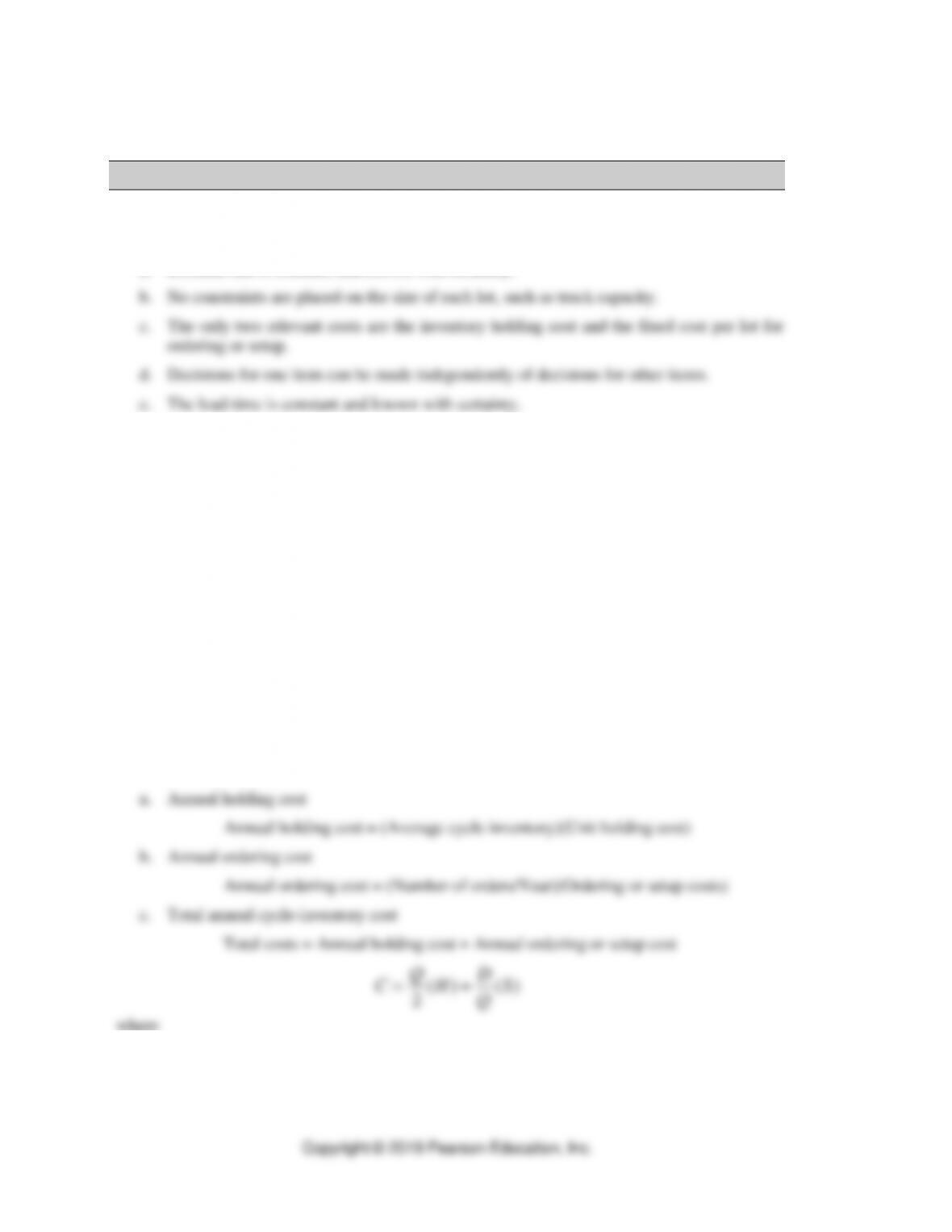
1. Five assumptions for the economic order quantity (EOQ)
a. Demand rate is constant and known with certainty.
2. Guidelines on when to use or modify the EOQ.
a. Don’t use the EOQ
• If you use the “make–to–order” strategy and your customer specifies the entire order
to be delivered in one shipment.
• If the order size is constrained.
b. Modify the EOQ
• If significant quantity discounts are given for larger lots.
• If replenishment of the inventory is not instantaneous (see Supplement D, “Special
Inventory Models”).
c. Use the EOQ
• If you follow a “make–to–stock” strategy and the item has relatively stable demand.
• If carrying costs and setup or ordering costs are known and relatively stable.
3. Calculating the EOQ
2S
Q
where
=C
total annual cycle-inventory cost
=Q
lot size, in units
=H
cost of holding one unit of inventory for a year, often expressed as a percentage of the
item’s value
=D
annual demand, in units per year
=S
cost of ordering or setting up one lot, in dollars per unit
• Note that the lowest cost occurs when the ordering cost is approximately equal to
holding cost. This is not by accident.
• A more efficient approach is to use the EOQ formula (derived from calculus).
2
OQ H
DS
E=
• Time between orders (TBO). Sometimes policies are expressed in terms of the time
between replenishments. TBO for a lot size is the elapsed time between receiving
orders of Q units.
( )
months/yr 12
EOQ
EOQ D
TBO =
• Finding the EOQ, Total Cost, and TBO. Use Application 9.1:
Suppose that you are reviewing the inventory policies on an $80 item stocked at a
hardware store. The current policy is to replenish inventory by ordering in lots of 360
units. Additional information is:
D = 60 units per week, or 3,120 units per year
S = $30 per order
H = 25% of selling price, or $20 per unit per year
What is the EOQ?
( )( )
97
20
30120,322 === H
DS
EOQ
units
What is the total annual cost of the current policy (Q = 360), and how does it compare
with the cost with using the EOQ?
Current policy
EOQ policy
360=Q
units
97=Q
units
( )( ) ( )( )
30360120,3202360 +=C
( )( ) ( )( )
3097120,320297 +=C
260600,3 +=C
965970 +=C
860,3$=C
935,1$=C
What is the time between orders (TBO) for the current policy and the EOQ policy,
expressed in weeks?
120,3
360
360 =TBO
(52 weeks per year) = 6 weeks
Copyright © 2019 Pearson Education, Inc.
120,3
97
=
EOQ
TBO
(52 weeks per year) = 1.6 weeks
• Tutor 9.3 in MyLab Operations Management provides a new example to practice the
application of the EOQ model.
• Active Model 9.1 in MyLab Operations Management provides additional insight on
the EOQ model and its uses.
4. Managerial insights from EOQ
a. A change in demand rate
• Because
D
is in the numerator, the EOQ increases in proportion to the square root of
the annual demand.
• When demand rises, the lot size also should rise, but more slowly than actual
demand.
b. A change in the order/setup costs
• Because
S
is in the numerator, increasing
S
increases the EOQ and, consequently,
the average cycle inventory.
• Conversely, reducing
S
reduces the EOQ, allowing smaller lot sizes to be produced
economically.
• This relationship explains why manufacturers are so concerned about reducing setup
time and costs. This is especially important for lean systems.
c. A change in the holding costs
• Because
H
is in the denominator, the EOQ declines when
H
increases.
• Conversely, when
H
declines, the EOQ increases.
• Larger lot sizes are justified by lower holding costs.
d. Errors in estimating
D
,
H
, and
S
.
• Total cost is fairly insensitive to errors, even when the estimates are wrong by a large
margin. The reasons are that errors tend to cancel each other out and that the square
root reduces the effect of the error.
6. Continuous Review System
Other names are: reorder point system (ROP) and fixed order quantity system
The focus is on inventory control systems for independent demand items.
Tracks inventory position (IP), which is the item’s ability to satisfy future demand
BOSROHIP −+=
where
=IP
inventory position
=OH
on-hand inventory
=SR
scheduled receipts (open orders)
=BO
units backordered

When the IP reaches a predetermined minimum level, called the reorder point (R), a fixed
quantity Q of the item is ordered.
Placing Orders with a Continuous Review System. Use Application 9.2:
The on-hand inventory is only 10 units, and the reorder point R is 100. There are no
backorders and one open order for 200 units. Should a new order be placed?
210020010 =−+=−+= BOSROHIP
R = 100
Decision: Place no new order.
1. Selecting the reorder point when demand and lead time are constant
a. Recall that safety stock inventory is inventory used to protect against uncertainties in
demand, lead time, and supply. When there are no uncertainties, there is no need for
safety stock.
b. The reorder point, R, equals demand during lead time. R = dL
2. Selecting the reorder point when demand is variable and lead time is constant
a. When there are uncertainties in demand, there is a need for safety stock.
b. The reorder point, R, is the average demand during lead time plus safety stock. R =
Ld
+
Safety Stock
where
=d
average demand per week (or day or month)
=L
constant lead time in weeks (or days or months)
c. As a management issue, the reorder point decision—based on judgment—to set a
reasonable service-level policy for the inventory and then determine the safety stock level
that satisfies this policy.
d. Three steps to arrive at a reorder point
• Step 1: Choose an appropriate service-level policy
Service level (or cycle-service level) is the desired probability of not running out
of stock in any one ordering cycle
The intent is to provide coverage over the protection period
• Step 2: Determine the demand during lead time probability distribution
Requires the specification of demand mean and demand standard deviation
Average demand during the lead time will be the sum of the averages for
each of the identical and independent distributions of demand..
The variance of the distribution of demand during lead time will be the
sum of the variances of identical and independent distributions of demand.
The standard deviation of the distribution of demand during lead time
is
2
dLT d d
LL
==
• Step 3: Determine the safety stock and reorder point levels
Assumes that demand during lead time is normally distributed.
The average demand during lead time is the centerline.
We compute the safety stock by multiplying the number of standard deviations
from the mean needed to implement the cycle-service level,
z
, by the standard
deviation of demand during lead time probability distribution,
dLT
:
dLT
z
stock Safety =
• The higher the value of
z
, the higher will be the safety stock and the cycle-service
level.
• Use Example 9.5 to demonstrate Reorder Point for Variable Demand and
Constant Lead Time
• Tutor 9.4 in MyLab Operations Management provides a new example to determine
the safety stock and the reorder point for a Q system.
• Selecting the Safety Stock and R. Use Application 9.3 to demonstrate the
calculations for safety stock and R in a Q system.
Suppose that the demand during lead time is normally distributed with an average of 85
and
dLT
= 40. Find the safety stock, and reorder point R, for a 95 percent cycle-
service level.
3. Selecting the reorder point when both demand and lead time are variable
a. In practice it is often the case that both the demand and lead time are variable.
b. The equations for safety stock and reorder points become more complicated.
c. The demand distribution and the lead time distribution are measured in the same units.
d. Demand and lead time are independent.
• Safety stock
dLT
z
=
• R = (Average weekly demand × Average lead time) + Safety stock
Ld=
+ Safety stock
where
=d
Average weekly (or daily or monthly) demand
=L
Average lead time
=
d
Standard deviation of weekly (or daily or monthly) demand
=
LT
Standard deviation of the lead time
=
dLT
2
2
2LTddL
+
• Use Example 9.7
• Reorder Point for Variable Demand and Variable Lead Time. Use Application 9.4.
(note this Solved Problem 6, part b)
Grey Wolf lodge is a popular 500-room hotel in the North Woods. Managers need to
keep close tabs on all of the room service items, including a special pint-scented bar
soap. The daily demand for the soap is 275 bars, with a standard deviation of 30
bars. Ordering cost is $10 and the inventory holding cost is $0.30/bar/year. The lead
time from the supplier is 5 days, with a standard deviation of 1 day. The lodge is
open 365 days a year.
What should the reorder point be for the bar of soap if management wants to have a
99 percent cycle-service?
Solution:
=d
275 bars
=L
5 days
=
d
30 bars
=
LT
1 day
=
dLT
( )( ) ( ) ( )
222
2
2
21275305+=+ LTddL
=283.06 bars
Consult the body of the Normal Distribution appendix for 0.9900, which corresponds
to a 99 percent cycle-service level. The closet value is 0.9901, which corresponds to
a z value of 2.33. We calculate the safety stock and reorder point as follows;
Safety stock
( )( )
06.28333.2 == dLT
z
= 659.53, or 660 bars
Reorder point
Ld=
+ safety stock = (275)(5) + 660 = 2,035 bars
4. Systems Based on the Q System
a. Two-Bin system
• Visual system
• An SKU’s inventory is stored at two different locations. Inventory is first withdrawn
from one bin. If the first bin is empty, the second bin provides backup to cover
demand until a replenishment order arrives.
• An empty first bin signals the need to place an order
b. Base-Stock System
• Issues a replenishment order, Q, each time a withdrawal is made, for the same
amount as the withdrawal.
• One-for-one replacement policy maintains the inventory position at a base-stock level
equal to expected demand during the lead time plus safety stock
5. Calculating total
Q
systems costs
a. Total cost = Annual cycle inventory holding cost + Annual ordering cost
+ Annual safety stock holding cost
b. Formula:
( ) ( )
)stockSafety )((
2HS
Q
D
H
Q
C++=
c. Continuous Review System: Putting It All Together. Use Application 9.5 to
demonstrate the complete specification of a Q system.
The Discount Appliance Store uses a continuous review system (Q system). One of the
company’s items has the following characteristics:
Demand = 10 units/wk (assume 52 weeks per year)
Ordering and setup cost (S) = $45/order
Holding cost (H) = $12/unit/year
Lead time (L) = 3 weeks (constant)
Standard deviation in weekly demand = 8 units
Cycle-service level = 70%
What is the total annual cost?
( ) ( ) ( )
42.845$12$845$
62
520
12$
2
62 =++=C
Suppose that the current policy is
Q
= 80 and R = 150. What will be the changes in
average cycle inventory and safety stock if your EOQ and R values are implemented?
Reducing
Q
from 80 to 62
Cycle inventory reduction = 40 – 31 = 9 units
Safety stock reduction = 120 – 8 = 112 units
Reducing R from 150 to 38
6. Advantages of the Q system
a. The review frequency of each item may be individualized.
b. Fixed lot sizes, if large enough, can result in quantity discounts.
c. Lower safety stocks results in savings.
7. Periodic Review System
Periodic review (
P
) system, sometimes called a fixed interval reorder system or periodic reorder
system.
Under a P system, four of the original EOQ assumptions are maintained.
No constraints are placed on the size of the lot.
The relevant costs are holding and ordering costs.
Decisions for one item are independent of decisions for other items.
Lead times are certain or supply is known.
When the predetermined time,
P
, has elapsed since the last review, an order is placed to
bring the inventory position up to the target inventory level,
T
.
Placing Orders with a Periodic Review System. Use Application 9.6:
The on-hand inventory is 10 units, and T is 400. There are no back orders, but one scheduled
receipt of 200 units. Now is the time to review. How much should be reordered?
210020010 =−+=−+= BOSROHIP
190210400 =−=− IPT
Decision: Order 190 units
1. Selecting the time between reviews
• Managers must make two decisions: the length of time between reviews,
P
and the
target inventory level,
T
.
2. Selecting a target inventory level when demand is variable and lead time is constant
a. The new order must be large enough to make the inventory position, IP, last beyond the
next review, which is P periods from now, but also for one lead time (L) after the next
review. IP must be enough to cover demand over a protection interval of P + L.
b. The average demand during the protection interval is
( )
LPd +
, or
( )
interval protectionfor stock Safety ++= LPdT
c. We compute safety stock for a
P
system much as we did for the
Q
system.
P+L
P+L
d+
Use example 9.9 to illustrate calculating P and T
3. Selecting the target inventory level when demand and lead time are variable.
• Using simulation is a practical approach.
• The Demand during the Protection Interval Simulator in OM Explorer can be used to
determine the distribution.
• Solved problem 6 demonstrates this approach.
4. Systems Based on the P System
• Single-Bin System
a maximum level is marked on the storage shelf or bin, and the inventory is
brought up to the mark periodically
• Optional Replenishment System
Sometimes called the optional review, min–max, or (s, S) system
It is used to review the inventory position at fixed time intervals and, if the
position has dropped to (or below) a predetermined level, to place a variable–
sized order to cover expected needs.
The new order is large enough to bring the inventory position up to a target
inventory, similar to T for the P system. However, orders are not placed after a
review unless the inventory position has dropped to the predetermined minimum
level.
5. Calculating total P system costs
• Total costs for the P system are the sum of the same three cost elements as for the Q
system, yet with differences in the calculation of the order quantity and the safety
stock.
• Formula:
( ) ( )
LP
HzS
dP
D
H
dP
C+
++=
2
b. Tutor 9.5 in MyLab Operations Management provides a new example to determine the
review interval and the target inventory for a P system.
c. Periodic Review System: Putting It All Together. Use Application 9.7 to show how to
construct a P-system and compare it to a Q-system.
Return to Discount Appliance Store (Application 9.5), but now use the P system for the item.
Previous information
Demand = 10 units/wk (assume 52 weeks per year) = 520
EOQ = 62 units (with reorder point system)
Lead time (L) = 3 weeks
Standard deviation in weekly demand = 8 units
z = 0.525 (for cycle-service level of 70%)