Chapter
4
Capacity Planning
DISCUSSION QUESTIONS
1. The primary economies of scale concern spreading the instructor’s salary over a
larger class and filling classrooms to capacity (and then some). Diseconomies occur
when additional help is required to review homework, administer tests, and
2. When demand for the drink is large enough, there are several ways that economies
of scale would benefit the boy. First, he can save on raw material costs. For
3. Answers will vary. By employing an expansionist strategy the firm attempts to stay
PROBLEMS
Planning Long-Term Capacity
1. Dahlia Medical Center
Labor room capacity = 30 rooms 3 days 24 hours/day = 2160 hours
Labor room utilization = (60 babies 24 hours/baby)/(2160 hours) = 66.67%
Capacity Planning ⚫ CHAPTER 4 ⚫
2. Capacity requirements in five years
3. Airline company
This year’s capacity requirement, allowing for a 25-percent capacity cushion, is 93.3 (or
4. Food Goblin Supermarket
a. Cashier availability = 4 persons x 5 days/week x 6 hours/day = 120 hours per week
Cashier utilization = (20 customers x .0833 hour x 30 hours/week)/ 120 = 41.7%
5. Food Goblin Supermarket, part 2
a. In order to maintain a 10% capacity cushion for cashiers:
(20 customers x 0.0833 hour x 30 hours/week) / (cashiers x 5 days/week x 6
hours/day) = 0.90 cushion. Thus; 49.98 / (30 x cashiers) = 0.90; solving for
cashiers = 1.85 or 2 cashiers.
b. In order to maintain a 10% capacity cushion for independent employees:
(20 customers x 0.2 hour x 30 hour/week) / (employees x 5 days/week x 6
hours/day) = 0.90 cushion, Thus; 120/ (30 x employees) = 0.90; solving for
A Systematic Approach to Long-Term Capacity Decisions
Capacity Planning ⚫ CHAPTER 4 ⚫
4-3
6. Purple Swift
The number of hours provided per machine is:
The capacity cushion is:
7. Macon Controls
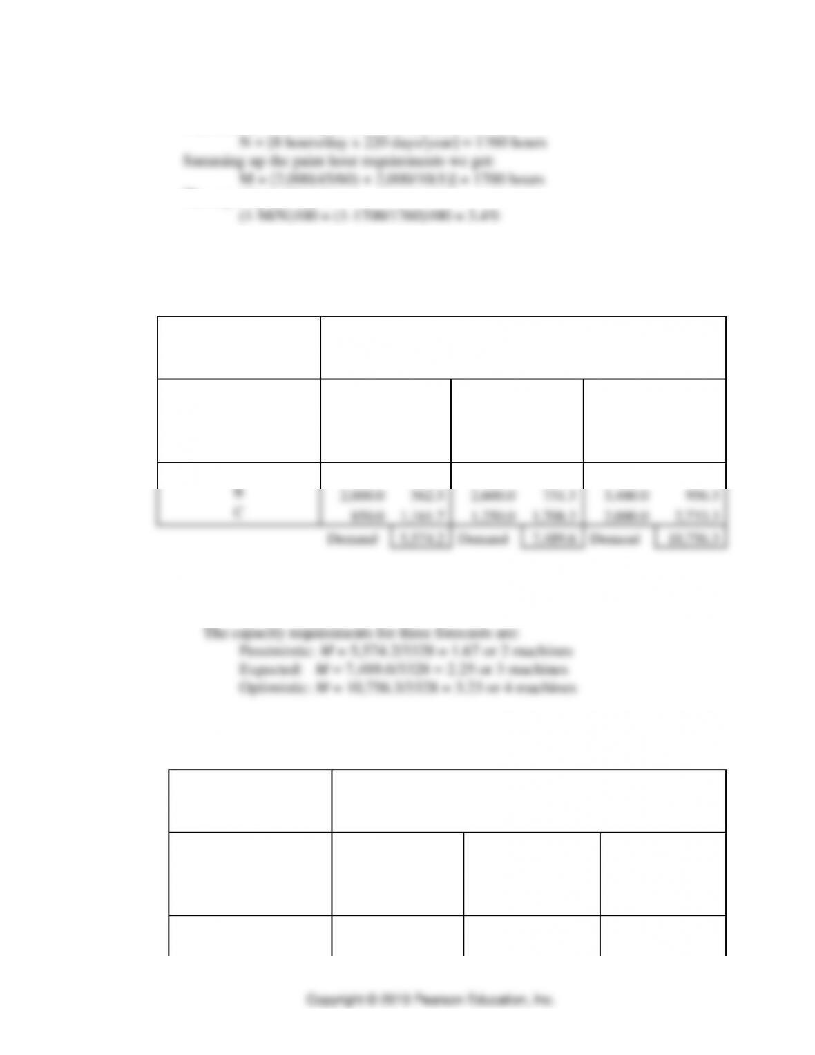
a. The total machine hour requirements for all three demand forecasts are
provided in the following Excel spreadsheet:
Capacity Information for
Macon Controls
Capacity Calculations
Control Unit
Pessimistic
Expected
Optimistic
Process
Time
(Dp)
Setup
Time
(D/Q)s
Process
Time
(Dp)
Setup
Time
(D/Q)s
Process
Time
(Dp)
Setup
Time
(D/Q)s
A
750.0
250.0
900.0
300.0
1,250.0
416.7
B
2,000.0
562.5
2,600.0
731.3
3,400.0
956.3
C
850.0
1,161.7
1,250.0
1,708.3
2,000.0
2,733.3
Demand
5,574.2
Demand
7,489.6
Demand
10,756.3
The number of hours (N) provided per machine is:
N = (2 shifts/day 8 hours/shift 5 days/week 52 weeks/year)(1.0 – 0.2)
= 3,328 hours/machine
b. The total machine hour requirements given that lot sizes are doubled are
provided in the following Excel spreadsheet:
Capacity Information for
Macon Controls
Capacity Calculations
Control Unit
Pessimistic
Expected
Optimistic
Process
Time
(Dp)
Setup
Time
(D/Q)s
Process
Time
(Dp)
Setup
Time
(D/Q)s
Process
Time
(Dp)
Setup
Time
(D/Q)s
A
750.0
125.0
900.0
150.0
1,250.0
208.3
B
2,000.0
281.3
2,600.0
365.6
3,400.0
478.1
Capacity Planning ⚫ CHAPTER 4 ⚫
C
850.0
580.8
1,250.0
854.2
2,000.0
1,366.7
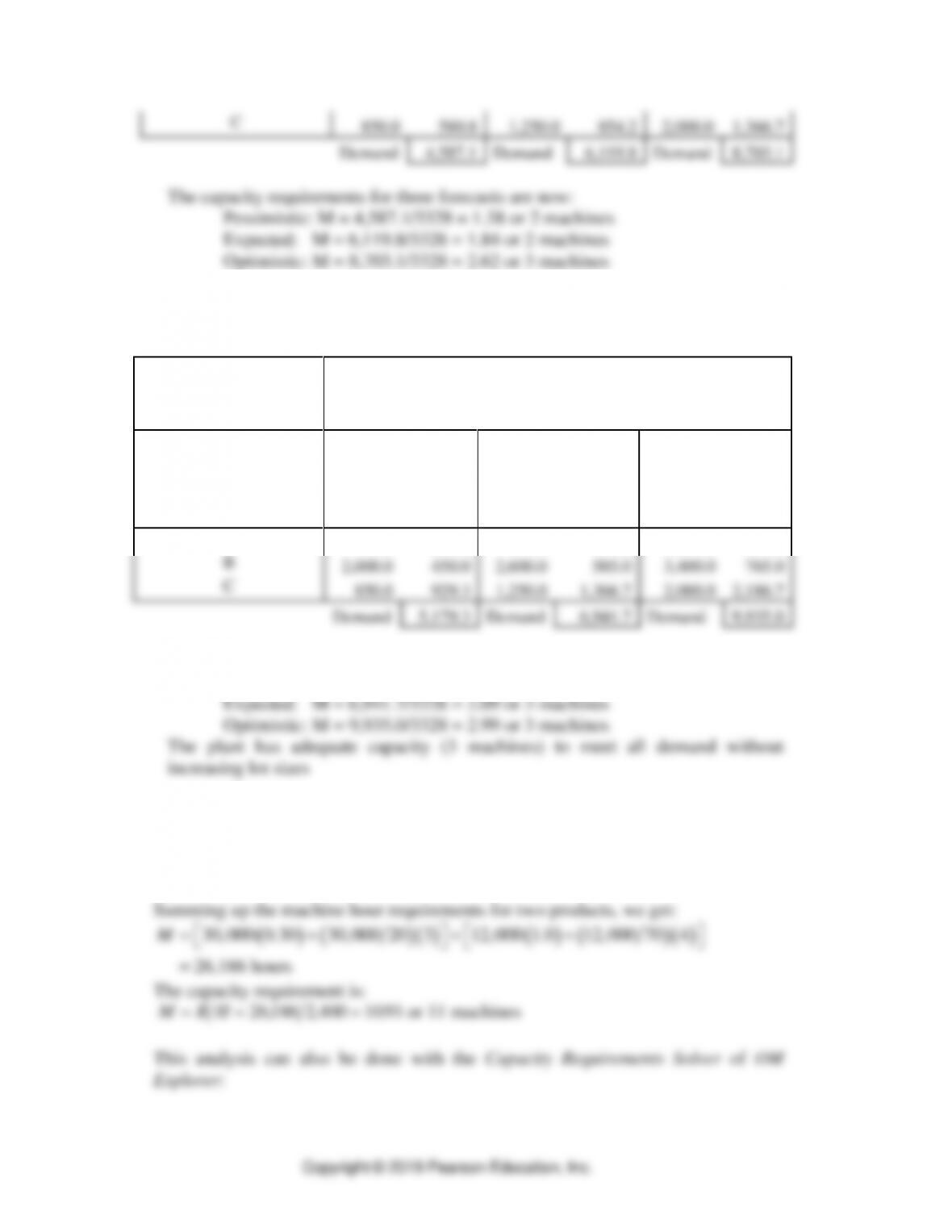
Demand
4,587.1
Demand
6,119.8
Demand
8,703.1
The capacity requirements for three forecasts are now:
Pessimistic: M = 4,587.1/3328 = 1.38 or 2 machines
Expected: M = 6,119.8/3328 = 1.84 or 2 machines
Optimistic: M = 8,703.1/3328 = 2.62 or 3 machines
c. The total machine hour requirements for all three demand forecasts given a 20%
setup time reduction follows:
Capacity Information for
Macon Controls
Capacity Calculations
Control Unit
Pessimistic
Expected
Optimistic
Process
Time
(Dp)
Setup
Time
(D/Q)s
Process
Time
(Dp)
Setup
Time
(D/Q)s
Process
Time
(Dp)
Setup
Time
(D/Q)s
A
750.0
200.0
900.0
240.0
1,250.0
333.3
B
2,000.0
450.0
2,600.0
585.0
3,400.0
765.0
C
850.0
929.3
1,250.0
1,366.7
2,000.0
2,186.7
Demand
5,179.3
Demand
6,941.7
Demand
9,935.0
The capacity requirements for three forecasts are now:
Pessimistic: M = 5,179.3/3328 = 1.56 or 2 machines
8. Up, Up and Away
The number of hours provided per machine is:
( )( )
2 shifts/day 8 hours/shift 200 days/year 3,200. 3,200 1 0.25
2, 400 hours/machine
NH= = = −
=
Capacity Planning ⚫ CHAPTER 4 ⚫
4-5
Processing Setup Lot Size Demand
Components (hr/unit) (hr/lot) (units/lot) Forecast
A 0.30 3.0 20 30,000
B 1.00 4.0 70 12,000
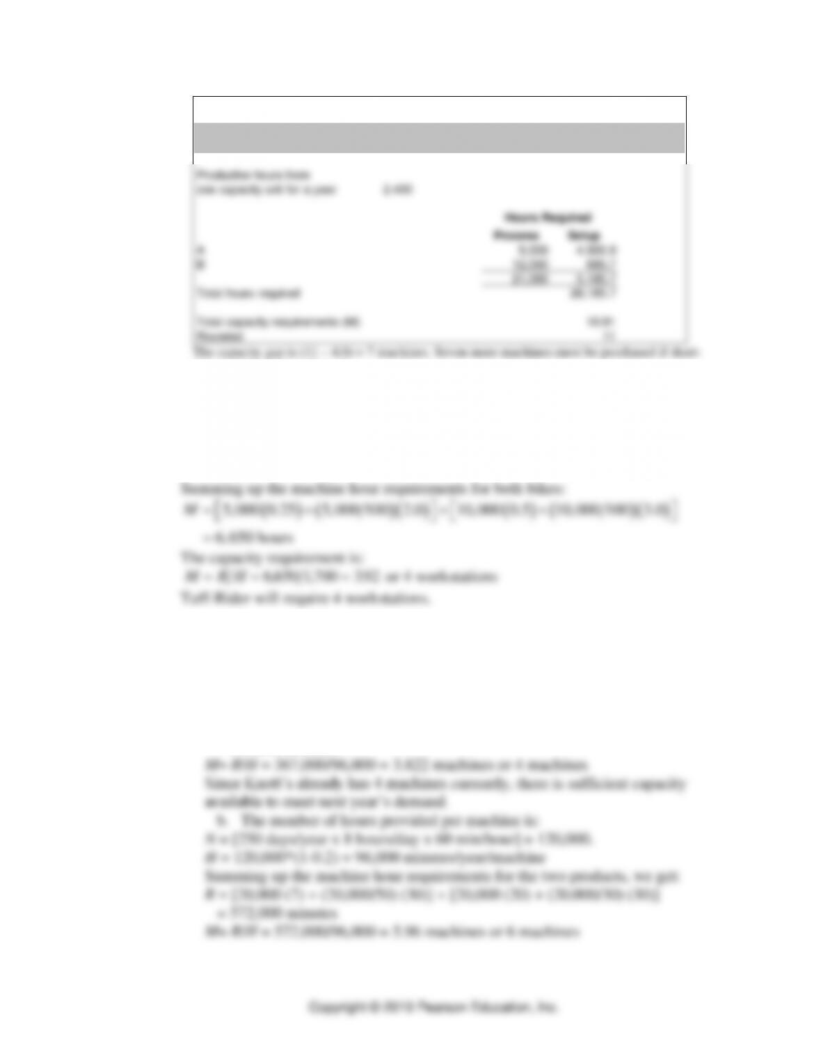
Productive hours from
one capacity unit for a year 2,400
Hours Required
Process Setup
A 9,000 4,500.0
B 12,000 685.7
21,000 5,185.7
Total hours required 26,185.7
Total capacity requirements (M) 10.91
Rounded 11
The capacity gap is (11 – 4.0) = 7 machines. Seven more machines must be purchased if short-
term options are not allowed.
9. Tuff-Rider
The number of hours (H) provided per workstation is
( )( )
8 hours/day 5days/week 50 weeks/year 2,000. 2,000 1.0 0.15
1,700 hours
NH= = = −
=
10. Knott’s Industries
a. The number of hours provided per machine is:
N = [250 days/year x 8 hours/day x 60 min/hour] = 120,000.
H = 120,000*(1-0.2) = 96,000 minutes/year/machine
Summing up the machine hour requirements for two products, we get:
R = [20,000 (7) + (20,000/50) (30)] + [10,000 (20) + (10,000/30) (45)]
= 367,000 minutes
Capacity Planning ⚫ CHAPTER 4 ⚫
Copyright © 2019 Pearson Education, Inc.
Even if the set-up time is reduced to 30 minutes for the super premium swing
sets, there is not enough capacity to produce 20,000 units of each type of swing
set since Knott’s has only 4 machines while 6 machines are required.
11. The French Prints of Arabelle
The solution is based on the assumption that sales vary in direct proportion to floor
area.
a. The last column in the table shows quarterly before-tax cash flows. The
first year’s $16,000 loss is followed by a $1,000 loss in the second year.
Sales
30% of
Incremental
Incremental
Incremental
Year
Quarter
($ per sf)
Sales
Quarterly
Salaries
Revenue
1000 sf
Rent
Minus Costs
1
1
$ 90.00
$27,000
$27,500
$12,000
($12,500)
2
$ 60.00
$18,000
$27,500
$ 8,000
($17,500)
3
$110.00
$33,000
$27,500
$12,000
($6,500)
4
$240.00
$72,000
$27,500
$24,000
$20,500
2
1
$ 99.00
$29,700
$27,500
$12,000
($9,800)
2
$ 66.00
$19,800
$27,500
$ 8,000
($15,700)
3
$121.00
$36,300
$27,500
$12,000
($3,200)
4
$264.00
$79,200
$27,500
$24,000
$27,700
b. The third year looks better. However, the $15,500 gain just about covers
the first year’s loss. Considering the time value of money would further
discourage this expansion.
Sales
30% of
Incremental
Incremental
Incremental
Year
Quarter
($ per sf)
Sales
Quarterly
Salaries
Revenue
1000 sf
Rent
Minus Costs
3
1
$108.90
$32,670
$27,500
$12,000
($6,830)
2
$ 72.60
$21,780
$27,500
$ 8,000
($13,720)
3
$133.10
$39,930
$27,500
$12,000
$430
4
$290.40
$87,120
$27,500
$24,000
$35,620
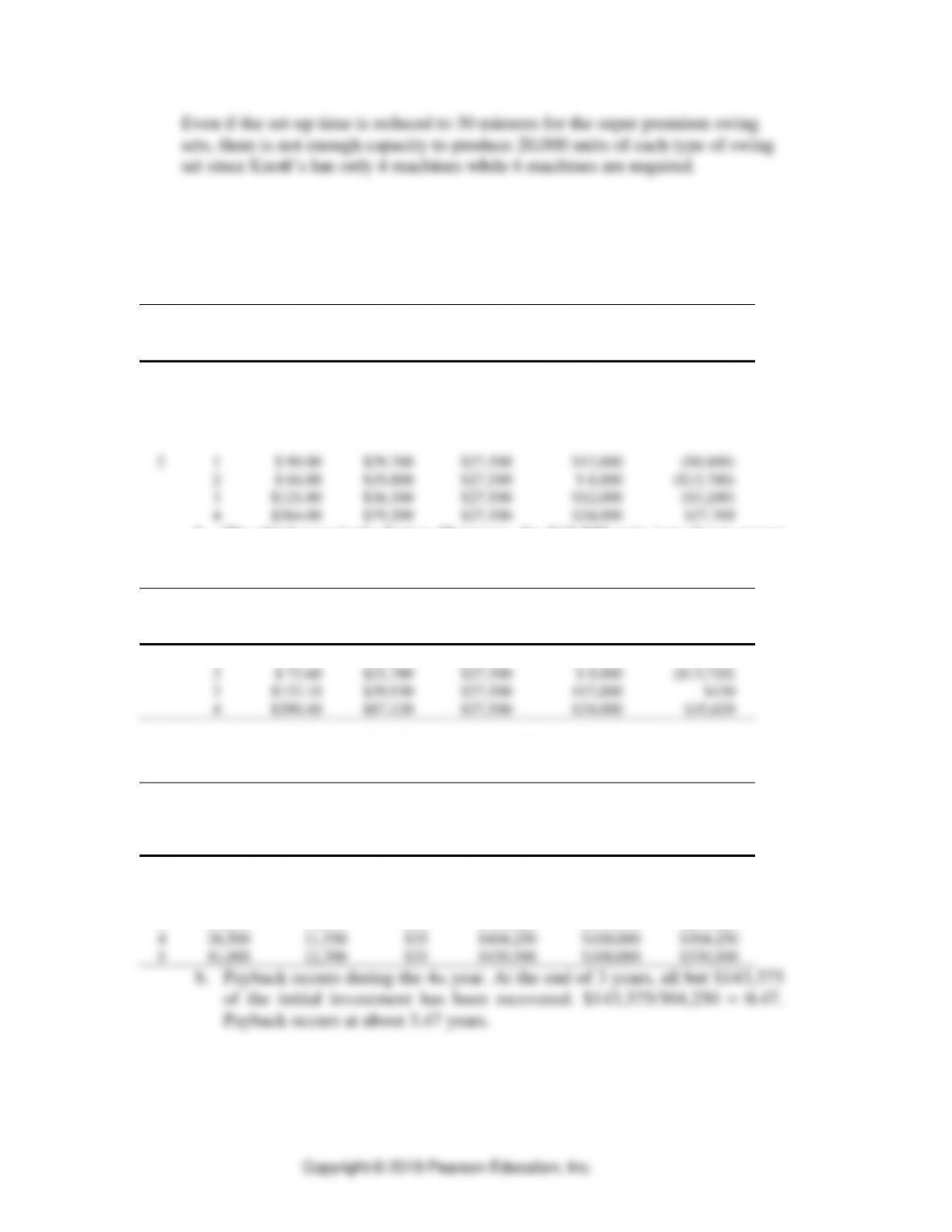
12. Astro World
a. The table shows incremental before-tax cash flows
Year
Projected
Attendance
Incremental
Attendance
(with
expansion)
Admis-
sion
Price
Incremental
Revenue
(with
expansion)
Investment
and
Operating
Costs
Cash Flow
0
$800,000
($800,000)
1
30,000
9,000
$30
$270,000
$100,000
$170,000
2
34,000
10,200
$30
$306,000
$100,000
$206,000
3
36,250
10,875
$35
$380,625
$100,000
$280,625
4
38,500
11,550
$35
$404,250
$100,000
$304,250
5
41,000
12,300
$35
$430,500
$100,000
$330,500
13. Kim Epson
Capacity of washing and drying station = (30 cars/hour) (12 hours/day)= 360
cars/day
Capacity Planning ⚫ CHAPTER 4 ⚫
4-7
Capacity of manual interior cleaning station = 200 cars/day
Incremental revenues (Friday, Saturday, and Sunday) from increasing capacity of
interior cleaning station to 300 cars will be:
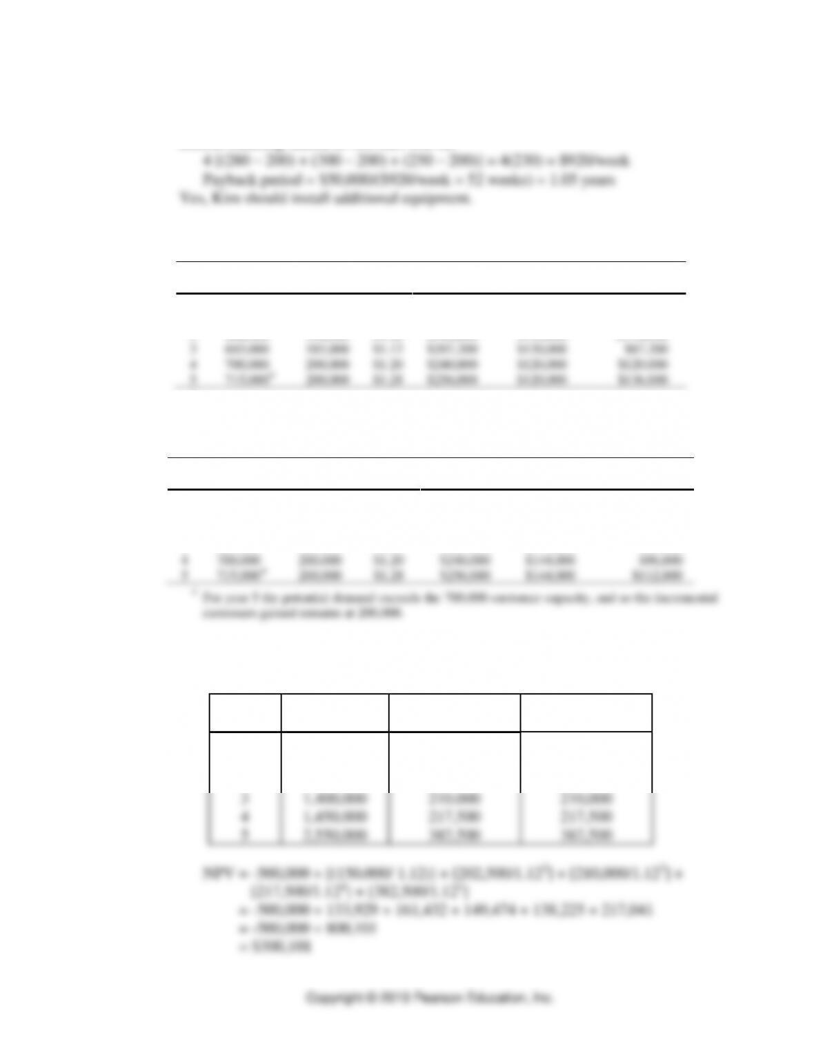
14. Roche Brothers
a. Expand to 700,000 capacity now.
Year
Customers
Incremental
Customers
2% of
Sales
Incremental
Revenue
Incremental
Costs & Rent
Incremental
Cash Flow
0
$200,000
($200,000)
1
560,000
60,000
$1.00
$60,000
$120,000
($60,000)
2
600,000
100,000
$1.06
$106,000
$120,000
($14,000)
3
685,000
185,000
$1.12
$207,200
$120,000
$87,200
4
700,000
200,000
$1.20
$240,000
$120,000
$120,000
5
715,000*
200,000
$1.28
$256,000
$120,000
$136,000
* For year 5 the potential demand exceeds the 700,000-customer capacity, and so the incremental
customers gained remains at 200,000.
b. Expand to 700,000 capacity, end of year 2.
Year
Customers
Incremental
Customers
2% of
Sales
Incremental
Revenue
Incremental
Costs & Rent
Incremental
Cash Flow
0
1
560,000
0
$1.00
$0
2
600,000
0
$1.06
$0
$240,000
($240,000)
3
685,000
185,000
$1.12
$207,200
$144,000
$63,200
4
700,000
200,000
$1.20
$240,000
$144,000
$96,000
5
715,000*
200,000
$1.28
$256,000
$144,000
$112,000
* For year 5 the potential demand exceeds the 700,000-customer capacity, and so the incremental
customers gained remains at 200,000.
15. MKM International
a. Machine 1 option:
Year
Projected
Cost
Savings with
New Machine 1
Cash Flow
0
($500,000)
1
1,000,000
150,000
150,000
2
1,350,000
202,500
202,500
3
1,400,000
210,000
210,000
4
1,450,000
217,500
217,500
5
2,550,000
382,500
382,500
Capacity Planning ⚫ CHAPTER 4 ⚫
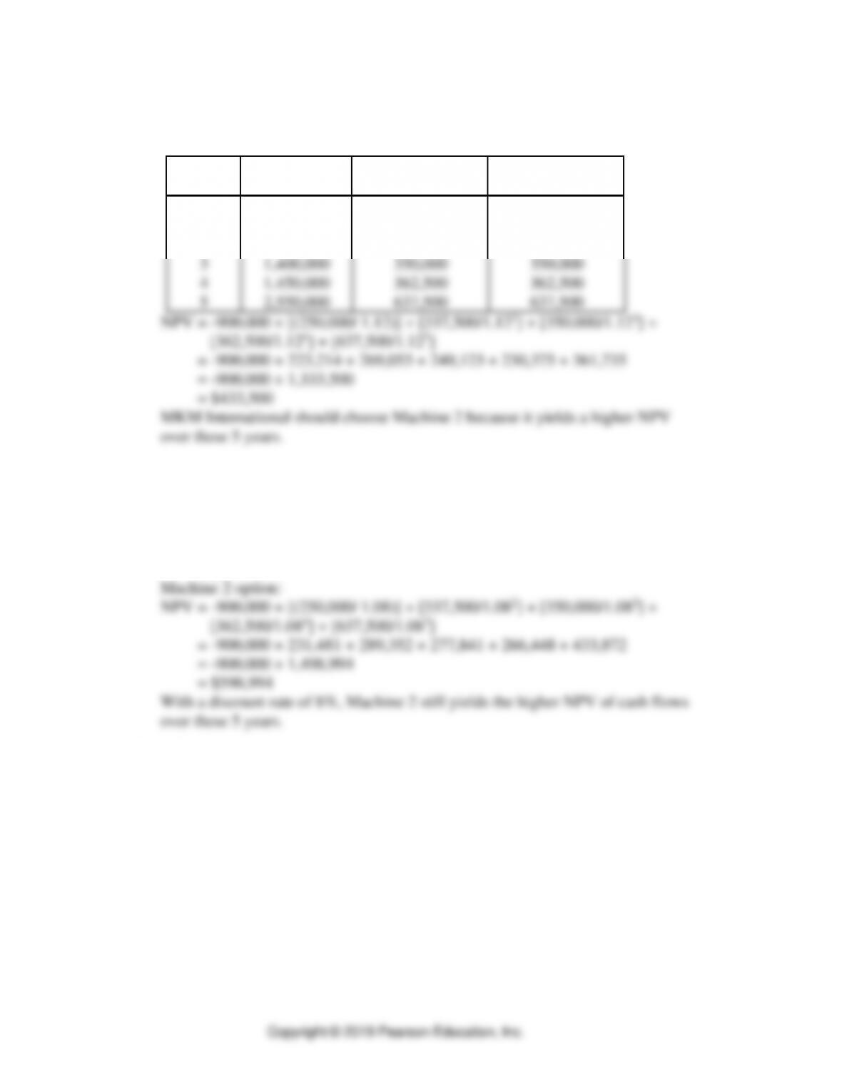
Machine 2 option:
Year
Projected
Cost
Savings with
New Machine 2
Cash Flow
0
($900,000)
1
1,000,000
250,000
250,000
2
1,350,000
337,500
337,500
3
1,400,000
350,000
350,000
4
1,450,000
362,500
362,500
5
2,550,000
637,500
637,500
b. Machine 1 option:
NPV = -500,000 + [(150,000/ 1.08)] + [202,500/1.082] + [210,000/1.083] +
[217,500/1.084] + [382,500/1.085]
= -500,000 + 138,889 + 173,611 + 166,705 + 159,869 + 260,323
= -500,000 + 899,397
= $399,397
16. River City
a. Alternative 1 (Al)
There must be an 80 million-gallon expansion now, which has a cash outflow of
$50 million. There are no other cash flows over the horizon.
Alternative 2 (A2)
There must be a 40 million-gallon expansion now (160–120) and another 40
million-gallon expansion (200–160) at the end of 10 years. These expansions
require a $30 million cash outflow at the end of years 0 and 10.
Alternative 3 (A3)
There must be a 20 million-gallon expansion at the end of years 0, 5, 10, 15.
Each expansion is accompanied by an $18 million cash outflow.
Capacity Planning ⚫ CHAPTER 4 ⚫
4-9
b. We will use the present value factors in Supplement F, “Financial
Analysis” in MyLab Operations Management to find the present value of
cash flows for each alternative.
Present Values (millions of dollars)
r = 12%
r = 16%
Al
$50
$50
A2
$30(1 + 0.3220) = $39.660
$30(1 + 0.2267) = $36.801
A3
$18(1 + 0.5674 + 0.3220 +
0.1827) = $37.298
$18(1 + 0.4761 + 0.2267 +
0.1079) = $32.593
At both extremes of the hurdle rate, Alternative 3 is the best.
c. The expansion probably requires a special bond issue, and it is probably
safer to go with an alternative that requires less of an outlay now (such as
Alternative 2 or 3).
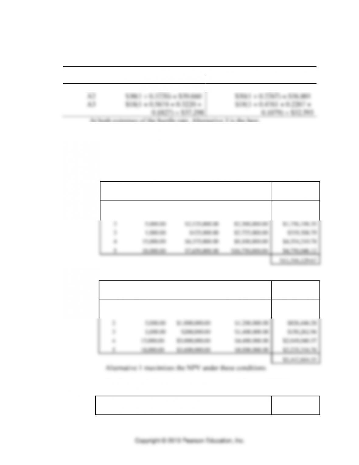
17. Mars Incorporated
a. The Excel spreadsheets below compute the cash flow and NPV for:
Alternative 1 assuming small increases in the cost of electrical power.
Year
Demand in
devices
Cash Inflow
(outflow)
Cumulative Cash
Inflow (outflow)
NPV at 10%
0
-$250,000.00
-$250,000.00
-$250,000.00
1
1,000.00
$425,000.00
$175,000.00
$386,363.64
2
5,000.00
$2,125,000.00
$2,300,000.00
$1,756,198.35
3
1,000.00
$425,000.00
$2,725,000.00
$319,308.79
4
15,000.00
$6,375,000.00
$9,100,000.00
$4,354,210.78
5
18,000.00
$7,650,000.00
$16,750,000.00
$4,750,048.12
$11,316,129.67
Alternative 2 assuming small increases in the cost of electrical power.
Year
Demand in
devices
Cash Inflow
(outflow)
Cumulative Cash
Inflow (outflow)
NPV at 10%
0
$0.00
$0.00
$0.00
1
1,000.00
$200,000.00
$200,000.00
$181,818.18
2
5,000.00
$1,000,000.00
$1,200,000.00
$826,446.28
3
1,000.00
$200,000.00
$1,400,000.00
$150,262.96
4
15,000.00
$3,000,000.00
$4,400,000.00
$2,049,040.37
5
18,000.00
$3,600,000.00
$8,000,000.00
$2,235,316.76
$5,442,884.55
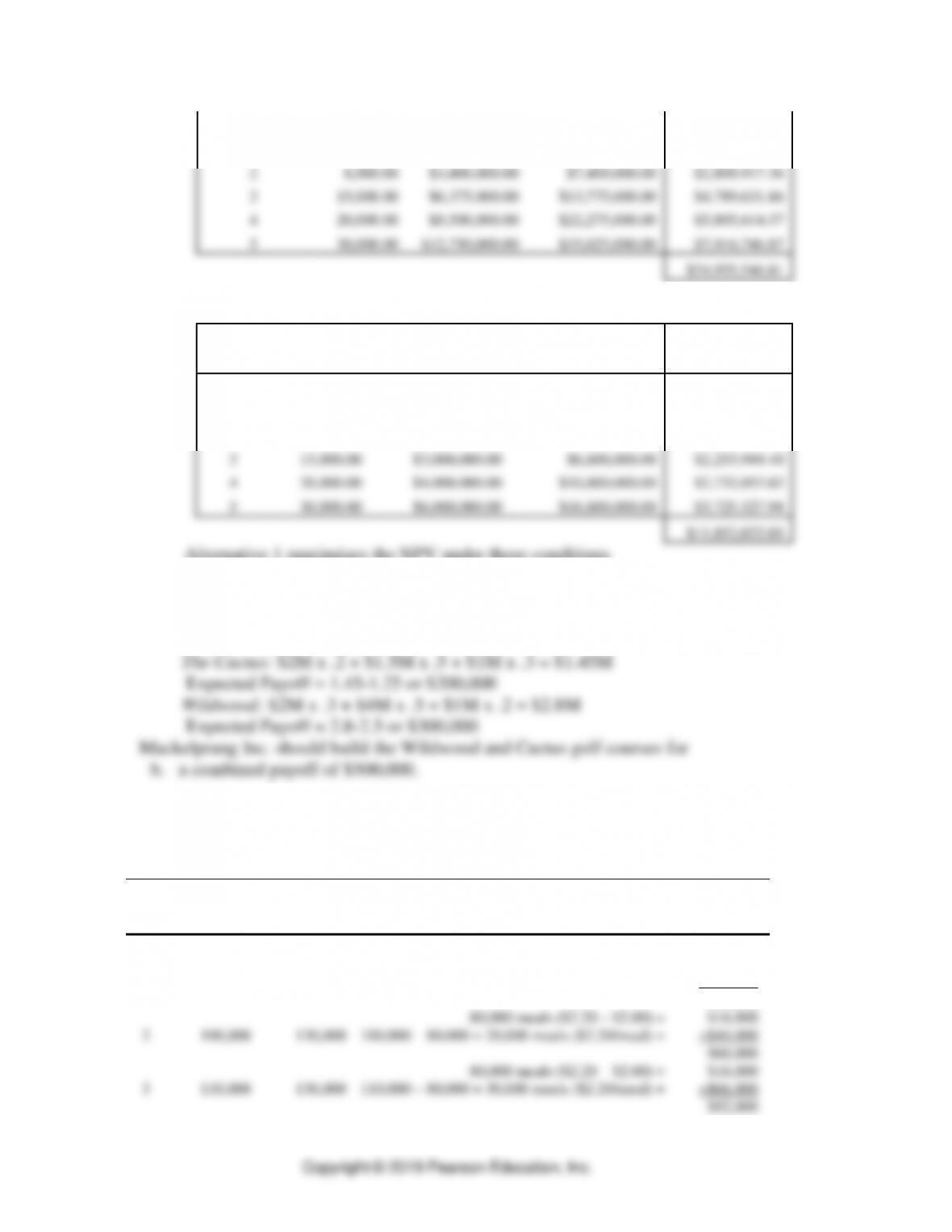
b. The Excel spreadsheets below compute the cash flow and NPV for:
Alternative 1 assuming large increases in the cost of electrical power.
Year
Demand in
devices
Cash Inflow
(outflow)
Cumulative Cash
Inflow (outflow)
NPV at 10%
Capacity Planning ⚫ CHAPTER 4 ⚫
0
-$250,000.00
-$250,000.00
-$250,000.00
1
10,000.00
$4,250,000.00
$4,000,000.00
$3,863,636.36
2
8,000.00
$3,400,000.00
$7,400,000.00
$2,809,917.36
3
15,000.00
$6,375,000.00
$13,775,000.00
$4,789,631.86
4
20,000.00
$8,500,000.00
$22,275,000.00
$5,805,614.37
5
30,000.00
$12,750,000.00
$35,025,000.00
$7,916,746.87
$24,935,546.81
Alternative 2 assuming large increases in the cost of electrical power.
Year
Demand in
devices
Cash Inflow
(outflow)
Cumulative Cash
Inflow (outflow)
NPV at 10%
0
$0.00
$0.00
$0.00
1
10,000.00
$2,000,000.00
$2,000,000.00
$1,818,181.82
2
8,000.00
$1,600,000.00
$3,600,000.00
$1,322,314.05
3
15,000.00
$3,000,000.00
$6,600,000.00
$2,253,944.40
4
20,000.00
$4,000,000.00
$10,600,000.00
$2,732,053.82
5
30,000.00
$6,000,000.00
$16,600,000.00
$3,725,527.94
$11,852,022.03
Alternative 1 maximizes the NPV under these conditions
18. Mackelprang Inc.
a. Indian river: $4M x .3 + $2.5M x .4 + $1M x .3 = $2.5M
Expected Payoff = 2.5-2.6 or -$100,000
19. Grandmother’s Chicken
Alternative 1: Expand both kitchen and dining area now to 130,000 capacity, cost
$336,000.
Projected
Projected
Calculation of Incremental Cash Flow
Cash Inflow
Year
Demand
Capacity
Compared to Base Case
(outflow)
(meals/year)
(meals/year)
80,000 meals/year
0
80,000
130,000
(336,000)
80,000 meals ($2.20 – $2.00) =
$16,000
1
90,000
130,000
90,000 – 80,000 = 10,000 meals ($2.20/meal) =
+$22,000
$38,000
80,000 meals ($2.20 – $2.00) =
$16,000
2
100,000
130,000
100,000 – 80,000 = 20,000 meals ($2.20/meal) =
+$44,000
$60,000
80,000 meals ($2.20 – $2.00) =
$16,000
3
110,000
130,000
110,000 – 80,000 = 30,000 meals ($2.20/meal) =
+$66,000
$82,000
Capacity Planning ⚫ CHAPTER 4 ⚫
4-11
80,000 meals ($2.20 – $2.00) =
$16,000
4
120,000
130,000
120,000 – 80,000 = 40,000 meals ($2.20/meal) =
+$88,000
$104,000
80,000 meals ($2.20 – $2.00) =
$16,000
5
130,000
130000
130,000 – 80,000 =50,000 meals ($2.20/meal) =
+$110,000
$126,000
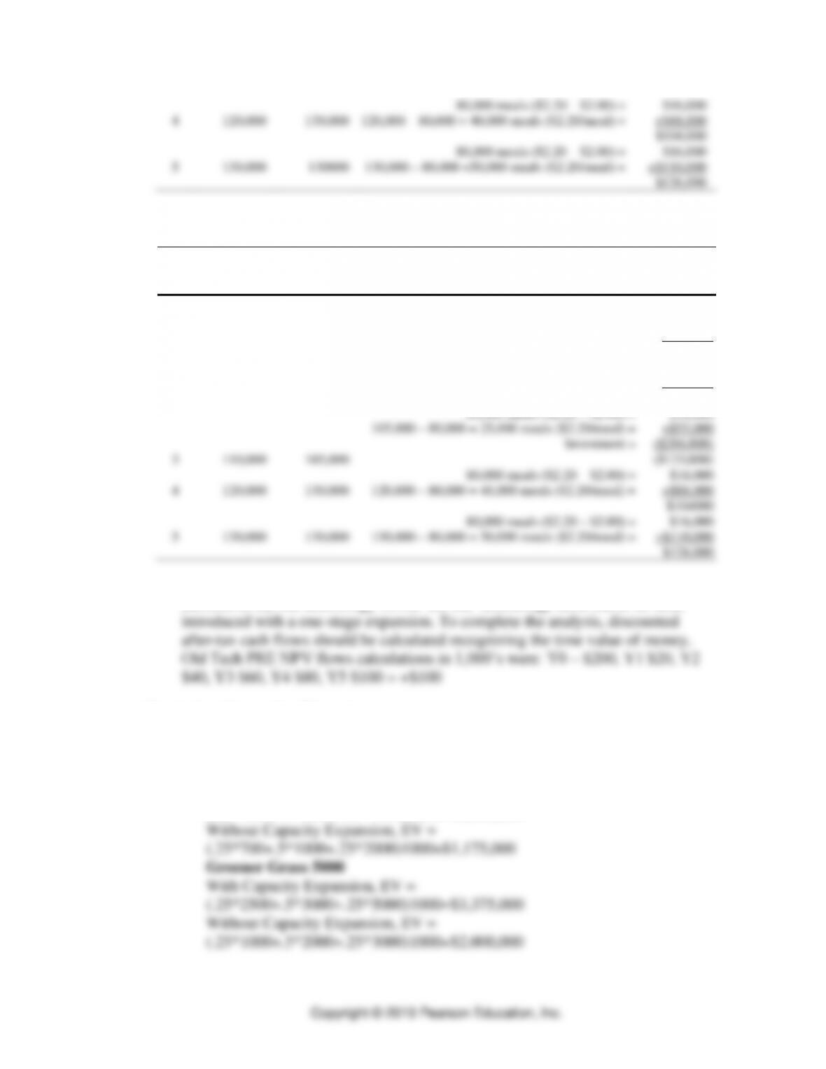
Alternative 2: Expand only kitchen now to 105,000 capacity, cost $220,000. At
end of Year 3, expand kitchen and dining to 130,000 capacity, cost $224,000.
Projected
Projected
Calculation of Incremental Cash Flow
Cash Inflow
Year
Demand
Capacity
Compared to Base Case
(outflow)
(meals/year)
(meals/year)
80,000 meals/year
0
80,000
105,000
Investment
(220,000)
80,000 meals ($2.20 – $2.00)=
$16,000
1
90,000
105,000
90,000 – 80,000 = 10,000 meals ($2.20/meal) =
+$22,000
$38,000
80,000 meals ($2.20 – $2.00) =
$16,000
2
100,000
105,000
100,000 – 80,000 = 20,000 meals ($2.20/meal) =
+$44,000
$60,000
80,000 meals ($2.20 – $2.00) =
$16,000
105,000 – 80,000 = 25,000 meals ($2.20/meal) =
+$55,000
Investment =
($204,000)
3
110,000
105,000
($133,000)
80,000 meals ($2.20 – $2.00) =
$16,000
4
120,000
130,000
120,000 – 80,000 = 40,000 meals ($2.20/meal) =
+$88,000
$104000
80,000 meals ($2.20 – $2.00) =
$16,000
5
130,000
130,000
130,000 – 80,000 = 50,000 meals ($2.20/meal) =
+$110,000
$126,000
Comparing just the sum of the cash flows for Alt. 1, $74,000 and Alt 2, −
$25,000 to the old technology flows, the old technology turns out to be best,
Tools for Capacity Planning
20. Dawson Electronics
a. Water Saver 1000
With Capacity Expansion, EV =
(.25*1000+.5*2000+.25*3000)1000=$2,000,000
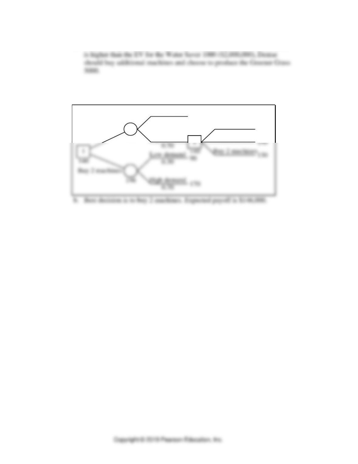
Capacity Planning ⚫ CHAPTER 4 ⚫
b. Since the expected value (EV) for the Greener Grass 5000 of $3,375,000
21. Purchasing one or two machines
a. Note: Payoffs are in $000s.
90
170
Low demand
0.30
High demand
0.70
120
1
146
134
146
Buy 2 machines
Buy 1 machine
Do nothing
Buy 2 machines
120
130
2
140
Low demand
0.30
High demand
0.70
Subcontract 140
Capacity Planning ⚫ CHAPTER 4 ⚫
4-13
22. Acme Steel Fabricators
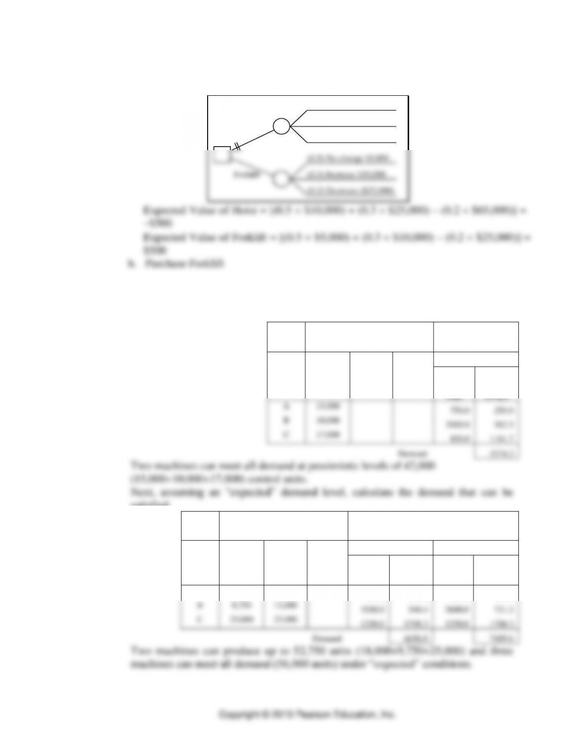
a. Decision tree
Forklift
Hoist
(0.5) No change $10,000
(0.3) Increase $25,000
(0.2) Decrease ($65,000)
(0.5) No change $5,000
(0.3) Increase $10,000
(0.2) Decrease ($25,000)
Expected Value of Hoist = [(0.5 $10,000) + (0.3 $25,000) – (0.2 $65,000)] =
–$500
Expected Value of Forklift = [(0.5 $5,000) + (0.3 $10,000) – (0.2 $25,000)] =
$500
b. Purchase Forklift
23. Macon Controls part 2
The Excel spreadsheet below calculates the total capacity required to meet
“pessimistic” demand.
Total Production Assuming
Pessimistic Demand
Capacity Required
Control
Unit
2
Machines
2 machines
Process
Time
(Dp)
Setup
Time
(D/Q)s
A
15,000
750.0
250.0
B
10,000
2000.0
562.5
C
17,000
850.0
1161.7
Demand
5574.2
Two machines can meet all demand at pessimistic levels of 42,000
(15,000+10,000+17,000) control units.
Next, assuming an “expected” demand level, calculate the demand that can be
satisfied.
Total Production Assuming
Expected Demand
Capacity Required
Control
Unit
2
Machines
3
Machines
2 Machines
3 Machines
Process
Time
(Dp)
Setup
Time
(D/Q)s
Process
Time
(Dp)
Setup
Time
(D/Q)s
A
18,000
18,000
900.0
300.0
900.0
300.0
B
9,750
13,000
1950.0
548.4
2600.0
731.3
C
25,000
25,000
1250.0
1708.3
1250.0
1708.3
Demand
6656.8
7489.6
Two machines can produce up to 52,750 units (18,000+9,750+25,000) and three
machines can meet all demand (56,000 units) under “expected” conditions.
Capacity Planning ⚫ CHAPTER 4 ⚫
Assuming “optimistic” demand, calculate the demand that can be satisfied.
Total Production Assuming
Optimistic Demand
Capacity Required
Control
Unit
2
Machines
3
Machines
4
Machines
2 Machines
3 Machines
4 Machines
Process
Time
(Dp)
Setup
Time
(D/Q)s
Process
Time
(Dp)
Setup
Time
(D/Q)s
Process
Time (Dp)
Setup Time
(D/Q)s
A
25,000
25,000
25,000
1250.0
416.7
1250.0
416.7
1250.0
416.7
B
1,000
14,000
17,000
200.0
56.3
2800.0
787.5
3400.0
956.3
C
40,000
40,000
40,000
2000.0
2733.3
2000.0
2733.3
2000.0
2733.3
Demand
6656.3
9987.5
10756.3
Two machines can produce up to 66,000 units (25,000+1,000+40,000), three
machines can produce up to 79,000 units (25,000+14,000+40,000), and four
machines can meet all demand (82,000 units) under “optimistic” conditions.
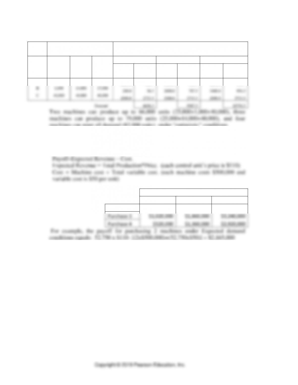
Using these production results, the Excel spreadsheet below provides the payoffs of
a decision to purchase 2, 3 or 4 machines under the three demand states of nature.
The calculation of each payoff proceeds as follows:
Payoff
Pessimistic
Expected
Optimistic
Purchase 2
$1,520,000
$2,165,000
$2,960,000
Purchase 3
$1,020,000
$1,860,000
$3,240,000
Purchase 4
$520,000
$1,360,000
$2,920,000
a. The decision tree
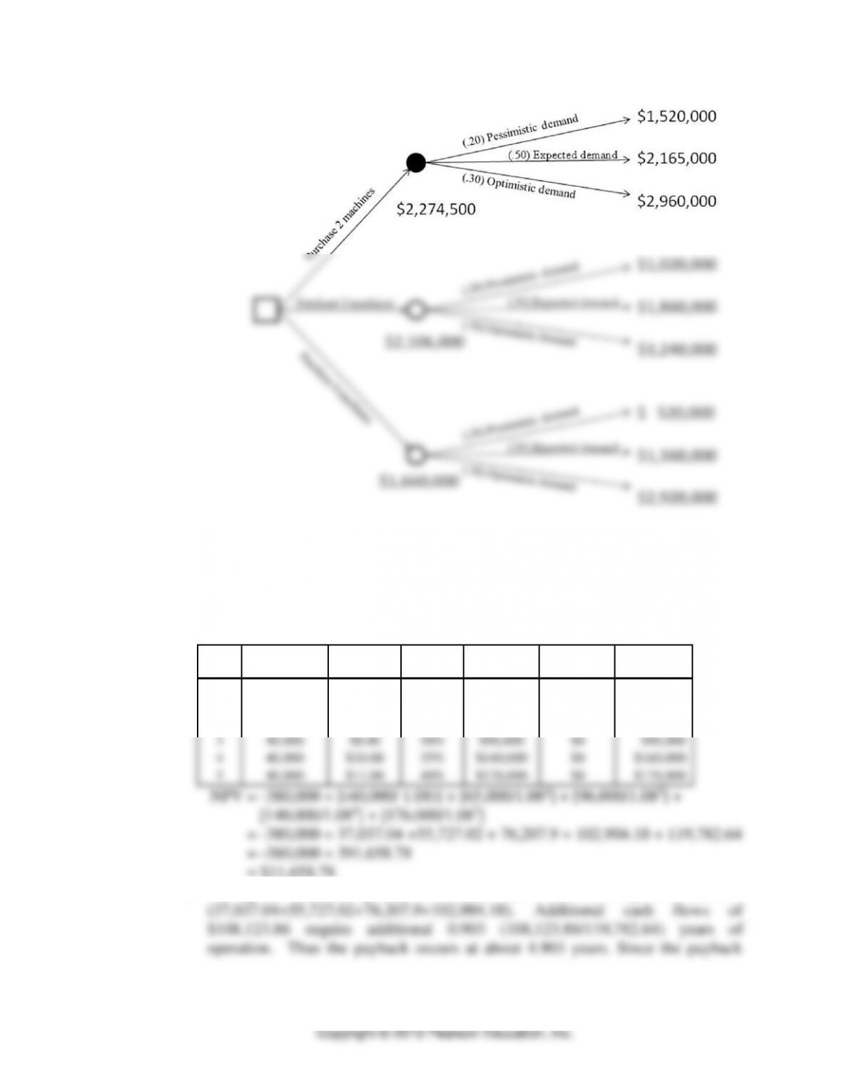
Capacity Planning ⚫ CHAPTER 4 ⚫
4-15
b. Using an Expected Value approach, the best decision is to purchase 2
machines with an expected payoff of $2,274,500.
24. Gas n’ Go
a.
Year
New
Customers
Sales Per
Customer
Profit
Margin
Profit
Costs
Cash Flow
0
$380,000
($380,000)
1
40,000
$5.00
20%
$40,000
$0
$40,000
2
40,000
$6.50
25%
$65,000
$0
$65,000
3
40,000
$8.00
30%
$96,000
$0
$96,000
4
40,000
$10.00
35%
$140,000
$0
$160,000
5
40,000
$11.00
40%
$176,000
$0
$176,000
NPV = -380,000 + [(40,000/ 1.08)] + [65,000/1.082] + [96,000/1.083] +
[140,000/1.084] + [176,000/1.085]
= -380,000 + 37,037.04 +55,727.02 + 76,207.9 + 102,904.18 + 119,782.64
= -380,000 + 391,658.78
= $11,658.78
b. During the first four years, incremental cash flows are only $ 271,876.14