14-1
Chapter
14
Supply Chain Integration
DISCUSSION QUESTIONS
1. Supply chain dynamics can be from internal sources or external sources. Dynamics
emanating from internal causes should be corrected by addressing the firm’s
policies on pricing and promotions, ability to provide correct data and information,
and the frequency of new service or product introductions, to name a few. Some of
2. Additive manufacturing (AM), is a term to describe the technologies that build
three-dimensional (3D) objects by adding layers of material such as plastic, metal,
or concrete. While AM has primarily been used to build prototypes during the
product development phase, it is now moving beyond its previous boundaries by
playing an integral part in manufacturing firms’ supply chains. AM has the ability to
impact (in fact disrupt) each of the four core supply chain processes. AM increases
production flexibility, enabling firms to reduce the time and resources necessary to
⚫ PART 3 ⚫ Managing Supply Chains
14-2
3. The experiences of GM and Chrysler are indicative of two differing approaches to
supplier relations. GM’s posture is indicative of a competitive orientation because
4. Firms with power in a supply relationship can influence the behavior of suppliers in
several ways. First, if there is an economic advantage because of the amount of
business the buyer gives to the supplier, the buyer can require the supplier to
participate in programs such as CFAR or to use technology such as RFID, for
5. Many firms have applied the principles of lean systems at the firm level to their
supply chains. Small lot sizes, close supplier ties, and quality at the source are all
applicable to a supply chain.
Small lot sizes. We have seen in our total cost analysis that lot sizes have an
impact on cycle inventory levels and freight costs because of the options
available to transport different quantities of product. Small lot sizes lower cycle
inventory requirements (perhaps enabling smaller warehouse space) while
Supply Chain Integration ⚫ CHAPTER 14 ⚫
14-3
PROBLEMS
Supplier Relationship Process
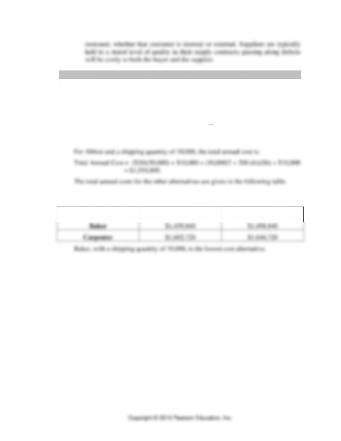
1. Horizon Cellular. We apply the equation for total annual cost analysis to each
supplier:
Total Annual Cost = pD + Freight costs + (Q/2 +
d
L)H + Administrative costs.
The average requirements per day are 200 circuit boards.
Shipping Quantity
10,000 25,000
Abbott
$1,554,800
$1,596,800
Baker
$1,459,840
$1,498,840
Carpenter
$1,602,720
$1,646,720
⚫ PART 3 ⚫ Managing Supply Chains
14-4
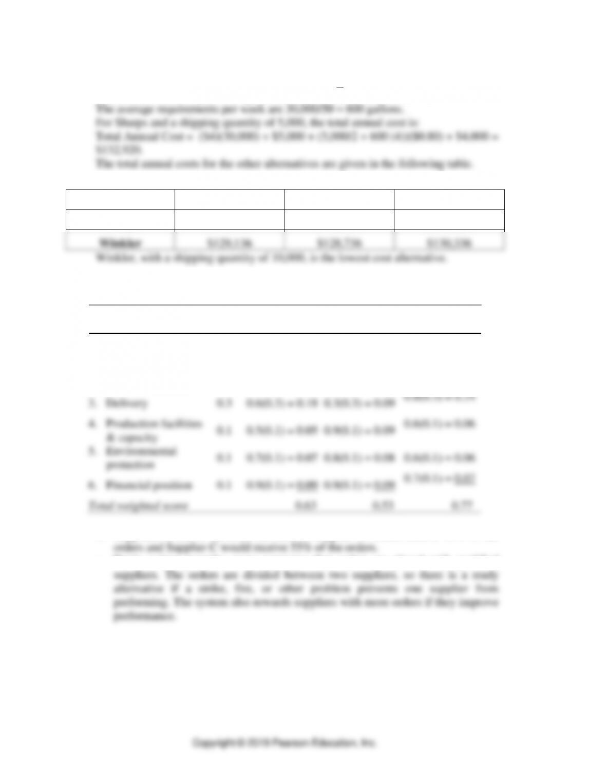
2. Eight Flags. We apply the equation for total annual cost analysis to each supplier:
Total Annual Cost = pD + Freight costs + (Q/2 +
d
L)H + Administrative costs.
Shipping Quantity
Supplier
5,000
10,000
15,000
Sharps
$132,920
$132,520
$133,920
Winkler
$129,136
$128,736
$130,336
3. Bennet
a. Each supplier’s performance can be calculated as:
Performance
Weighted Rating
Criterion
Weight
Supplier A
Supplier B
Supplier C
1. Price
0.2
0.6(0.2) = 0.12
0.5(0.2) = 0.10
0.9(0.2) = 0.18
2. Quality
0.2
0.6(0.2) = 0.12
0.4(0.2) = 0.08
0.8(0.2) = 0.16
3. Delivery
0.3
0.6(0.3) = 0.18
0.3(0.3) = 0.09
0.8(0.3) = 0.24
4. Production facilities
& capacity
0.1
0.5(0.1) = 0.05
0.9(0.1) = 0.09
0.6(0.1) = 0.06
5. Environmental
protection
0.1
0.7(0.1) = 0.07
0.8(0.1) = 0.08
0.6(0.1) = 0.06
6. Financial position
0.1
0.9(0.1) = 0.09
0.9(0.1) = 0.09
0.7(0.1) = 0.07
Total weighted score
0.63
0.53
0.77
b. Suppliers A and C survived the hurdle. Supplier A would receive 45% of the
c. Ben’s system provides some assurance that orders are placed with qualified
Supply Chain Integration ⚫ CHAPTER 14 ⚫
14-5
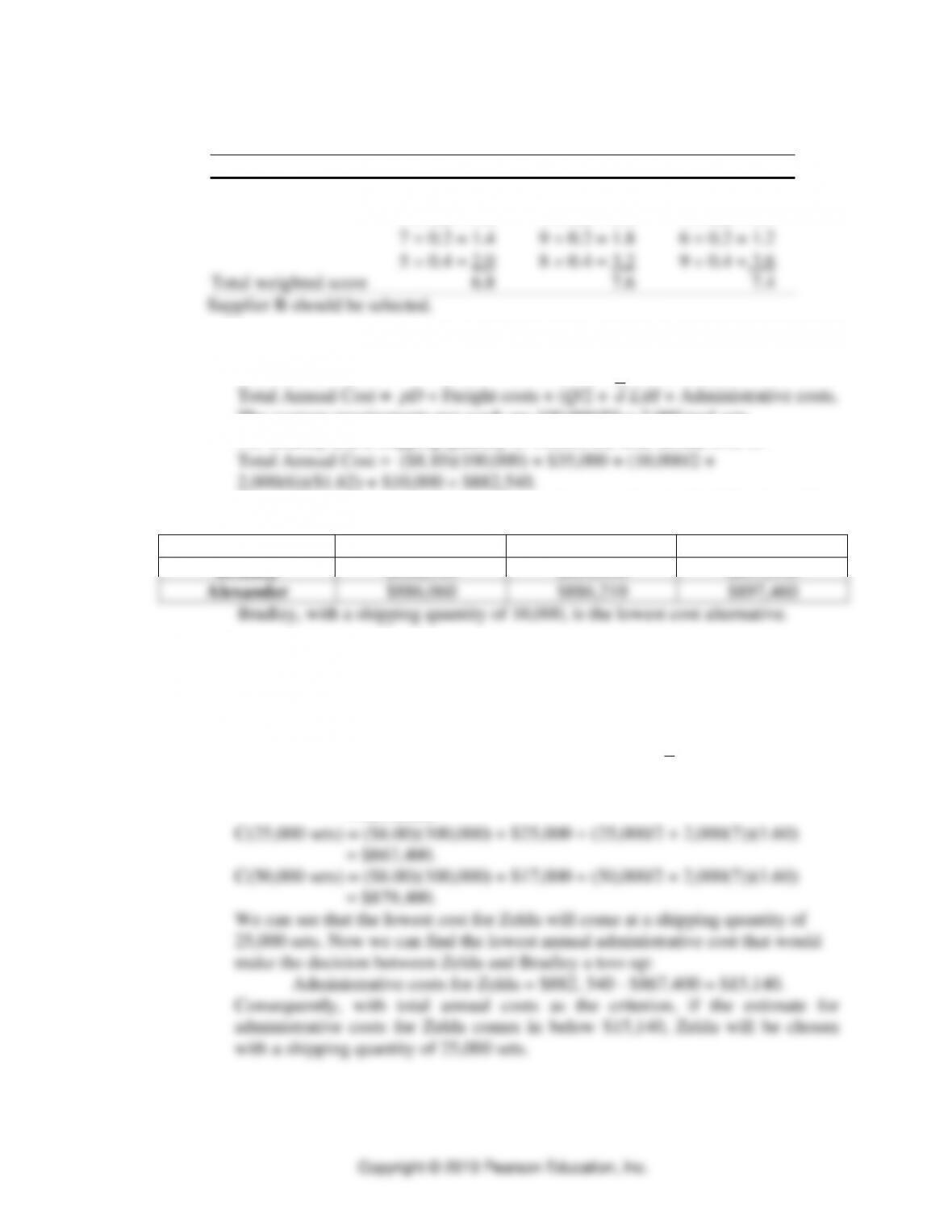
4. Beagle Clothiers. The weights for the four criteria—price, quality, delivery, and
flexibility—should be 0.2, 0.2, 0.2, and 0.4, respectively. The weighted scores are
Supplier A
Supplier B
Supplier C
8 0.2 = 1.6
6 0.2 = 1.2
6 0.2 = 1.2
9 0.2 = 1.8
7 0.2 = 1.4
7 0.2 = 1.4
7 0.2 = 1.4
9 0.2 = 1.8
6 0.2 = 1.2
5 0.4 = 2.0
8 0.4 = 3.2
9 0.4 = 3.6
Total weighted score
6.8
7.6
7.4
Supplier B should be selected.
5. Weekend Projects.
a. We apply the equation for total annual cost analysis to each supplier:
The average requirements per week are 100,000/50 = 2,000 tool sets.
For Bradley and a shipping quantity of 10,000, the total annual cost is:
The total annual costs for the other alternatives are given in the following table.
Shipping Quantity
Supplier
10,000
25,000
50,000
Bradley
$882,540
$884,690
$897,940
Alexander
$886,060
$886,210
$897,460
b. The target indifference point is $882,540, which is Bradley’s lowest cost.
However, the best shipping size for Zelda may not be 10,000 tools sets as it was
for Bradley. Consequently, each shipping quantity must be evaluated for Zelda.
We begin by finding the total annual costs for Zelda for each shipping quantity
without the annual administrative costs.
C(Q sets) = pD + Freight costs + (Q/2 +
d
L)H
C(10,000 sets) = ($8.00)(100,000) + $45,000 + (10,000/2 + 2,000(7))(1.60)
= $875,400.
⚫ PART 3 ⚫ Managing Supply Chains
14-6
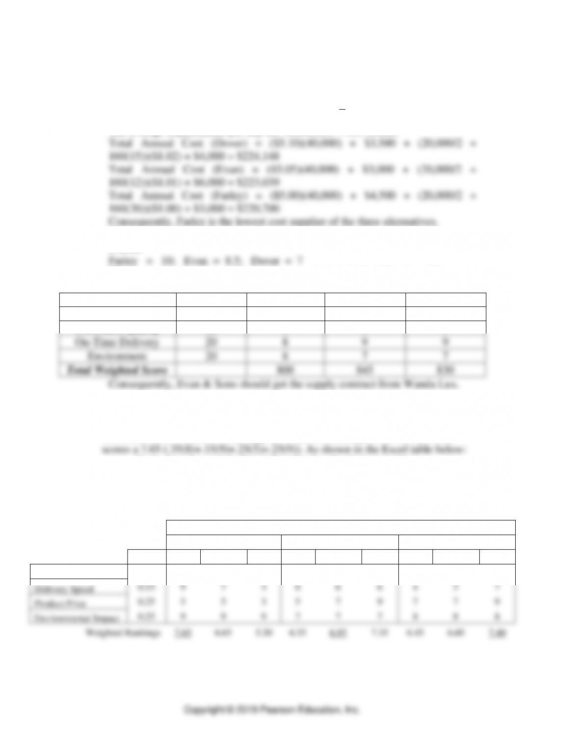
6. Wanda Lux.
a. We first determine the total annual cost for each supplier using the following
equation:
Total Annual Cost = pD + Freight costs + (Q/2 +
d
L)H + Administrative costs.
The average requirements per day are 40,000/250 = 160 bottles.
b. We can now rank the three suppliers with regard to total annual cost and assign
a score:
The weighted scores for each supplier are contained in the following table:
Performance Score
Criterion
Weight
Dover
Evan
Farley
Total Cost
30
7
8.5
10
Consistent Quality
30
9
9
7
On-Time Delivery
20
8
9
9
Environment
20
8
7
7
Total Weighted Score
800
845
830
Consequently, Evan & Sons should get the supply contract from Wanda Lux.
7. Adelie Enterprises
a. For each supplier at each demand level, multiply each criterion by the supplier’s
score and sum. Thus, the local supplier under the assumption of low demand
Under low demand the Local Supplier has the highest ranking
Under moderate demand the National Supplier has the highest ranking
Under high demand the International Supplier has the highest ranking
Supplier Rating Under Low, Moderate and High Levels of Demand
Local Supplier
National Supplier
International Supplier
Weight
Low
Moderate
High
Low
Moderate
High
Low
Moderate
High
Product Quality
0.35
8
6
5
7
7
7
6
6
6
Delivery Speed
0.15
9
7
3
6
6
6
4
5
7
Product Price
0.25
5
5
3
5
7
9
7
7
9
Environmental Impact
0.25
9
9
9
7
7
7
8
8
8
Weighted Rankings
7.65
6.65
5.20
6.35
6.85
7.35
6.45
6.60
7.40
b. Using a maximin decision criterion, the company would select the
International Supplier. This supplier’s smallest ranking (6.45 under low
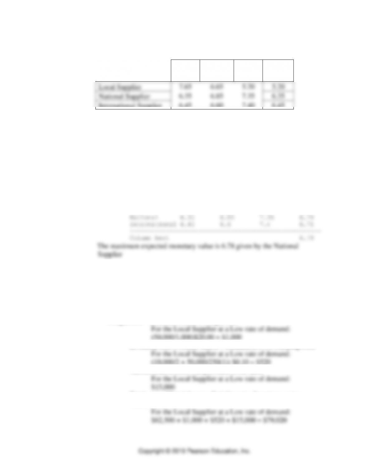
Supply Chain Integration ⚫ CHAPTER 14 ⚫
14-7
demand) is greater than the Local Supplier’s (5.20 at high demand) and the
National Supplier’s (6.35 under low demand).
Low
Moderate
High
Min
Ranking
Local Supplier
7.65
6.65
5.20
5.20
National Supplier
6.35
6.85
7.35
6.35
International Supplier
6.45
6.60
7.40
6.45
c. For each supplier, multiply the probability of each demand level with the
supplier’s ranking at that demand level and sum. For example, the expected
ranking for the local supplier is 6.71 (.35(7.65) +.45(6.65)+.20(5.2)).
The following POM for Windows Decision Analysis printout provides the
solution to which supplier achieves the highest expected ranking
Module/submodel: Decision Making/Decision Tables
Results ———-
Expected
Low Moderate High Value
—————————————————–
Probabilities .35 .45 .2
Local 7.65 6.65 5.2 6.71
8. Adelie Enterprises part 2.
d. The total costs for the local supplier at a low level of demand are assessed as
follows:
Material cost = Demand x unit price
For the Local Supplier at a Low rate of demand:
50,000($1.25) = $62,500
Freight cost = Demand/10,000 x Freight cost
Inventory cost = (Order Size/2 + Demand/250 ) x Carrying Cost
(10,000/2 + 50,000/250(1)) $0.10 = $520
Administrative Cost = as provided in the table
Total cost = Material cost + Freight cost + Inventory cost +
Administrative Cost
⚫ PART 3 ⚫ Managing Supply Chains
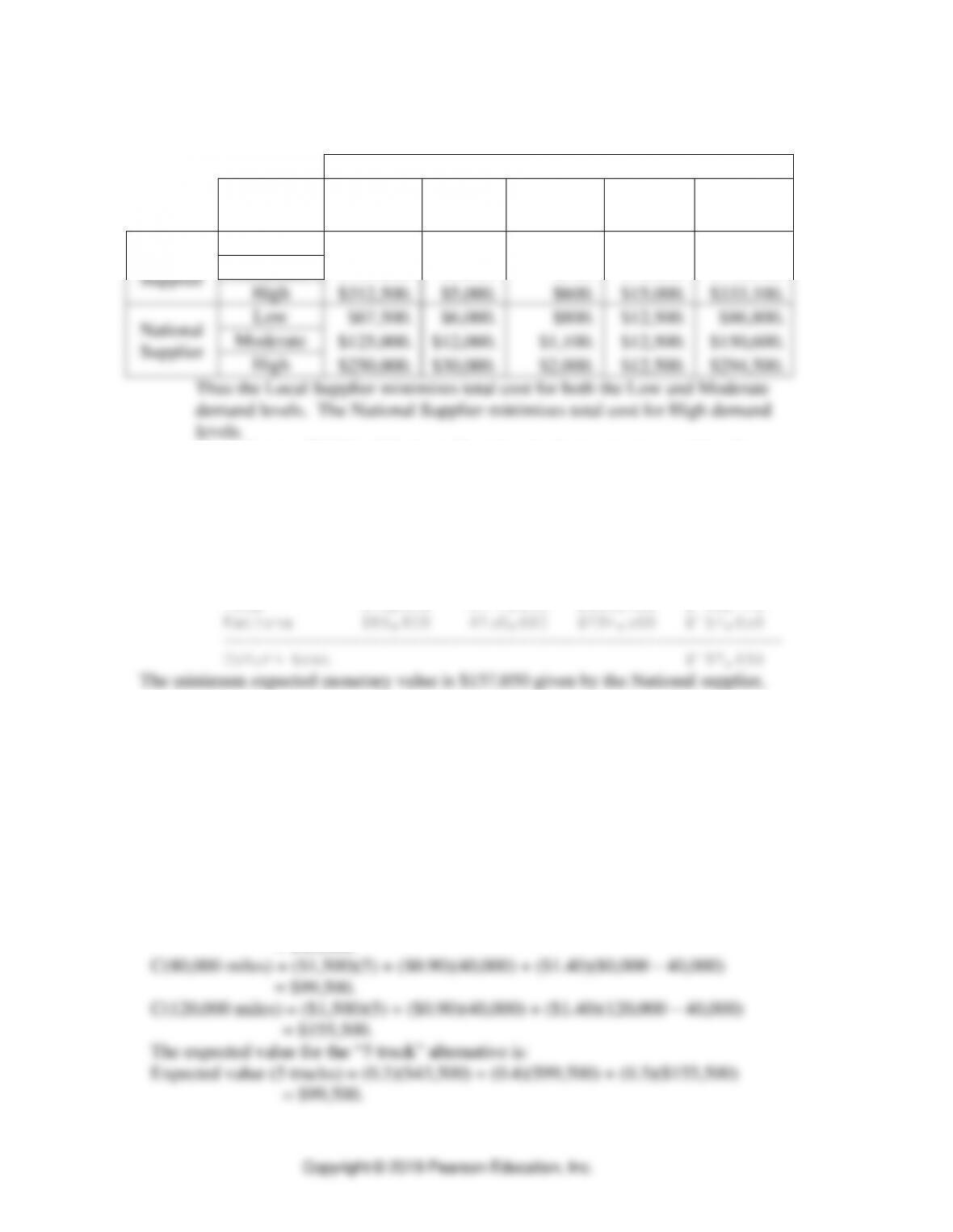
14-8
The following Excel Table provides cost calculations of both suppliers across
all levels of demand.
Costs
Demand
Level
Material
Cost
Freight
Cost
Inventory
Cost
Admin
Cost
Total Cost
Local
Supplier
Low
$62,500.
$1,000.
$520.
$15,000.
$79,020.
Moderate
$125,000.
$2,000.
$540.
$15,000.
$142,540.
High
$312,500.
$5,000.
$600.
$15,000.
$333,100.
National
Supplier
Low
$67,500.
$6,000.
$800.
$12,500.
$86,800.
Moderate
$125,000.
$12,000.
$1,100.
$12,500.
$150,600.
High
$250,000.
$30,000.
$2,000.
$12,500.
$294,500.
e. The following POM for Windows Decision Analysis printout provides the
solution to which supplier achieves the lowest expected cost.
Module/submodel: Decision Making/Decision Tables
Results ———-
Expected
Low Moderate High Value
—————–—————–———–————
Probabilities .35 .45 .2
Local $79,020 $142,540 $333,100 $158,420
Order Fulfillment Process
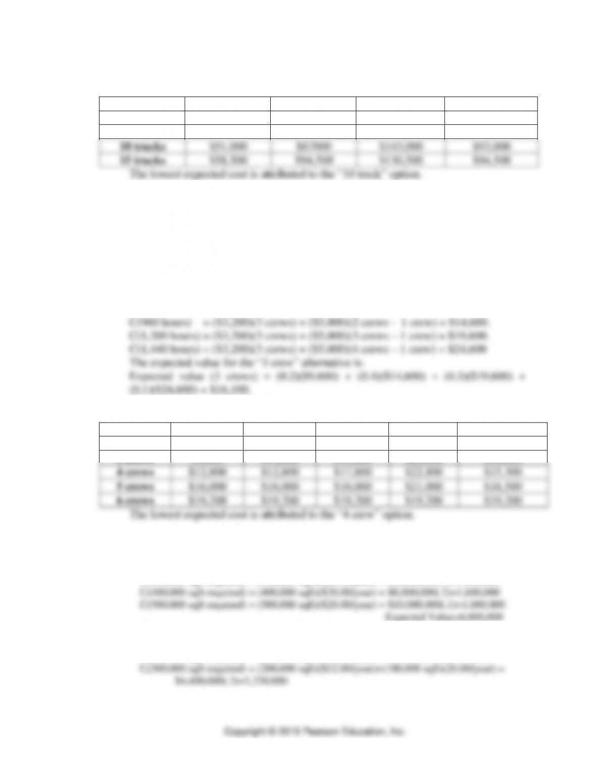
9. Wingman Distributing. We use the expected value decision rule. Management has
identified three potential levels of demand for the trucks and three corresponding
levels of capacity. Consequently, there are three cost possibilities for each capacity
level. Costs include the capital costs, variable costs, and rental costs, if applicable.
The expected value of a capacity alternative is the probability of a level of demand
multiplied by the cost for that level of demand, summed over all possible levels of
demand. Take for example the “5 truck” alternative:
C(40,000 miles) = ($1,500)(5) + ($0.90)(40,000)
= $43,500.
Supply Chain Integration ⚫ CHAPTER 14 ⚫
14-9
The expected values for all alternatives are:
Probabilities
0.3
0.4
0.3
Alternatives
40,000 miles
80,000 miles
120,000 miles
Expected Value
5 trucks
$43,500
$99,500
$155,500
$99,500
10 trucks
$51,000
$87000
$143,000
$93,000
15 trucks
$58,500
$94,500
$130,500
$94,500
10. Sanchez Trucking. We use the expected value decision rule. Management has
identified four potential levels of demand for teams and four corresponding levels of
capacity. Consequently, there are four cost possibilities for each capacity
alternative. Costs include the wages and benefits for the teams to be on the payroll
and the cost of using short-term employees to cover for capacity shortages. The
expected value of an alternative is the probability of a level of demand times the
corresponding cost if that demand materializes, summed over all possible levels of
demand. Take for example the “3 team” alternative:
C(720 hours) = ($3,200)(3 crews) = $9,600.
The expected values for all alternatives are:
Probabilities
0.2
0.4
0.3
0.1
Alternatives
720 hours
960 hours
1,200 hours
1,440 hours
Expected Value
3 crews
$9,600
$14,600
$19,600
$24,600
$16,100
4 crews
$12,800
$12,800
$17,800
$22,800
$15,300
5 crews
$16,000
$16,000
$16,000
$21,000
$16,500
6 crews
$19,200
$19,200
$19,200
$19,200
$19,200
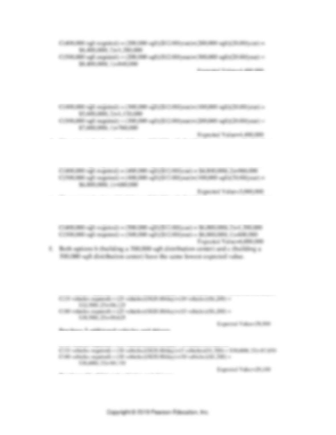
11. Acadia Logistics
a. The expected value of not building a distribution center is calculated as follows:
C(200,000 sqft required) = (200,000 sqft)($20.00/year) = $4,000,000(.4)=1,600,000
C(300,000 sqft required) = (300,000 sqft)($20.00/year) = $6,000,000(.3)=1,800,000
b. The expected value of building a 200,000 sqft distribution center is calculated as
follows:
C(200,000 sqft required) = (200,000 sqft)($12.00/year) = $2,400,000(.4)=960,000
⚫ PART 3 ⚫ Managing Supply Chains
14–10
Expected Value=4,400,000
c. The expected value of building a 300,000 sqft distribution center is calculated as
follows:
C(200,000 sqft required) = (300,000 sqft)($12.00/year) = $3,600,000(.4)=1,440,000
C(300,000 sqft required) = (300,000 sqft)($12.00/year) = $3,600,000(.3)=1,080,000
d. The expected value of building a 400,000 sqft distribution center is calculated as
follows:
C(200,000 sqft required) = (400,000 sqft)($12.00/year) = $4,800,000(.4)=1,920,000
C(300,000 sqft required) = (400,000 sqft)($12.00/year) = $4,800,000(.3)=1,440,000
e. The expected value of building a 500,000 sqft distribution center is calculated as
follows:
C(200,000 sqft required) = (500,000 sqft)($12.00/year) = $6,000,000(.4)=2,400,000
C(300,000 sqft required) = (500,000 sqft)($12.00/year) = $6,000,000(.3)=1,800,000
12. Transworld Deliveries: the expected value of each hiring decision follows:
Purchase no additional vehicles and drivers
C(25 vehicles required) = (25 vehicles)($820.00/day) =$20,500(.25)=$5,125
C(30 vehicles required) = (25 vehicles)($820.00/day)+(5 vehicles)($1,200) = $26,500(.25)=$6,625
Purchase 5 additional vehicles and drivers
C(25 vehicles required) = (30 vehicles)($820.00/day) =$24,600(.25)=$6,150
C(30 vehicles required) = (30 vehicles)($820.00/day) = $24,600(.25)=$6,150
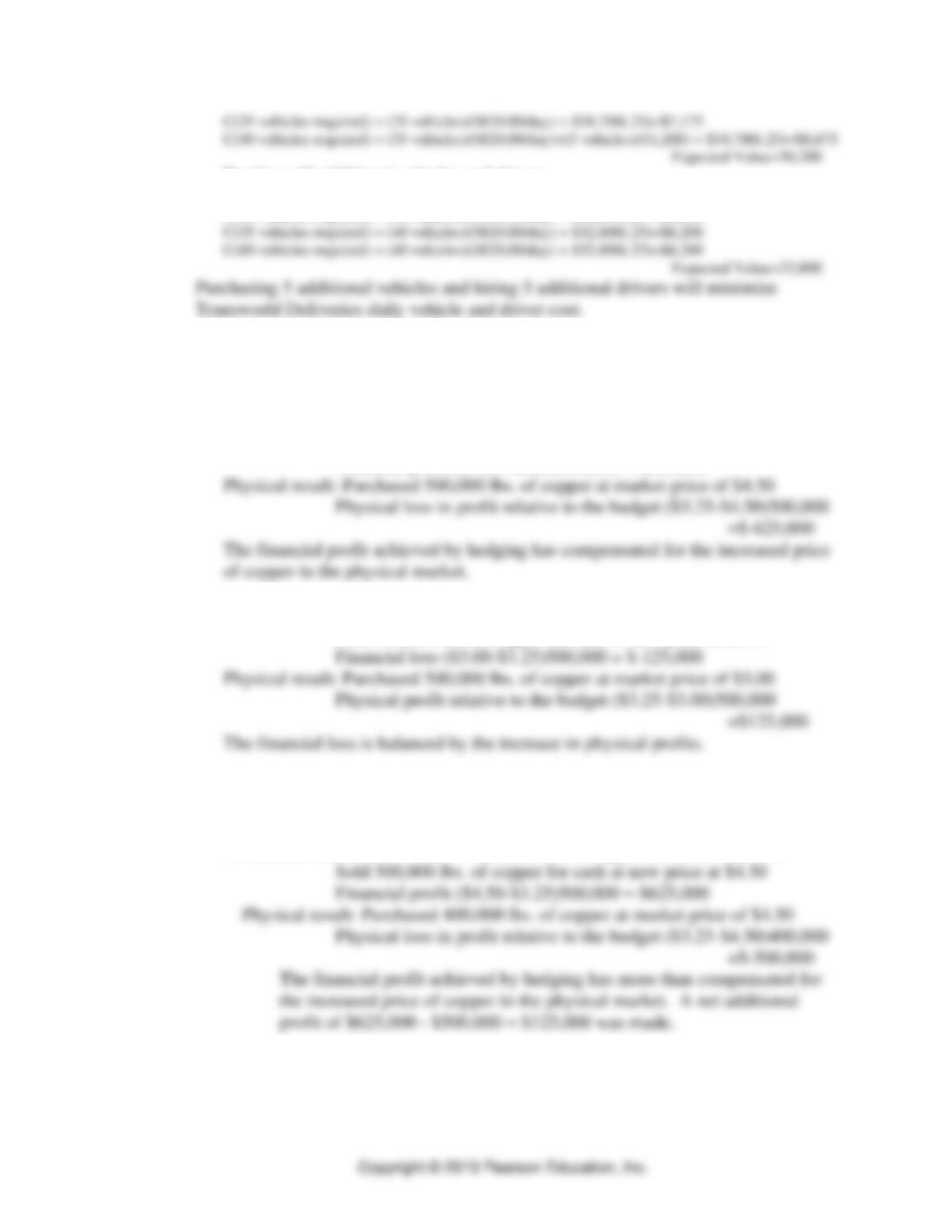
Purchase 10 additional vehicles and drivers
C(25 vehicles required) = (35 vehicles)($820.00/day) =$28,700(.25)=$7,175
C(30 vehicles required) = (35 vehicles)($820.00/day) = $28,700(.25)=$7,175
Supply Chain Integration ⚫ CHAPTER 14 ⚫
14–11
Purchase 15 additional vehicles and drivers
C(25 vehicles required) = (40 vehicles)($820.00/day) =$32,800(.25)=$8,200
C(30 vehicles required) = (40 vehicles)($820.00/day) = $32,800(.25)=$8,200
Supply Chain Risk Management
13. Eastmark
a. Financial result: Paid $3.25 for 500,000 lbs. of copper on futures contract
Sold 500,000 lbs. of copper for cash at new price of $4.50
Financial profit ($4.50-$3.25)500,000 = $625,000
b. Financial result: Paid $3.25 for 500,000 lbs. of copper on futures contract
Sold 500,000 lbs. of copper for cash at new price at $3.00
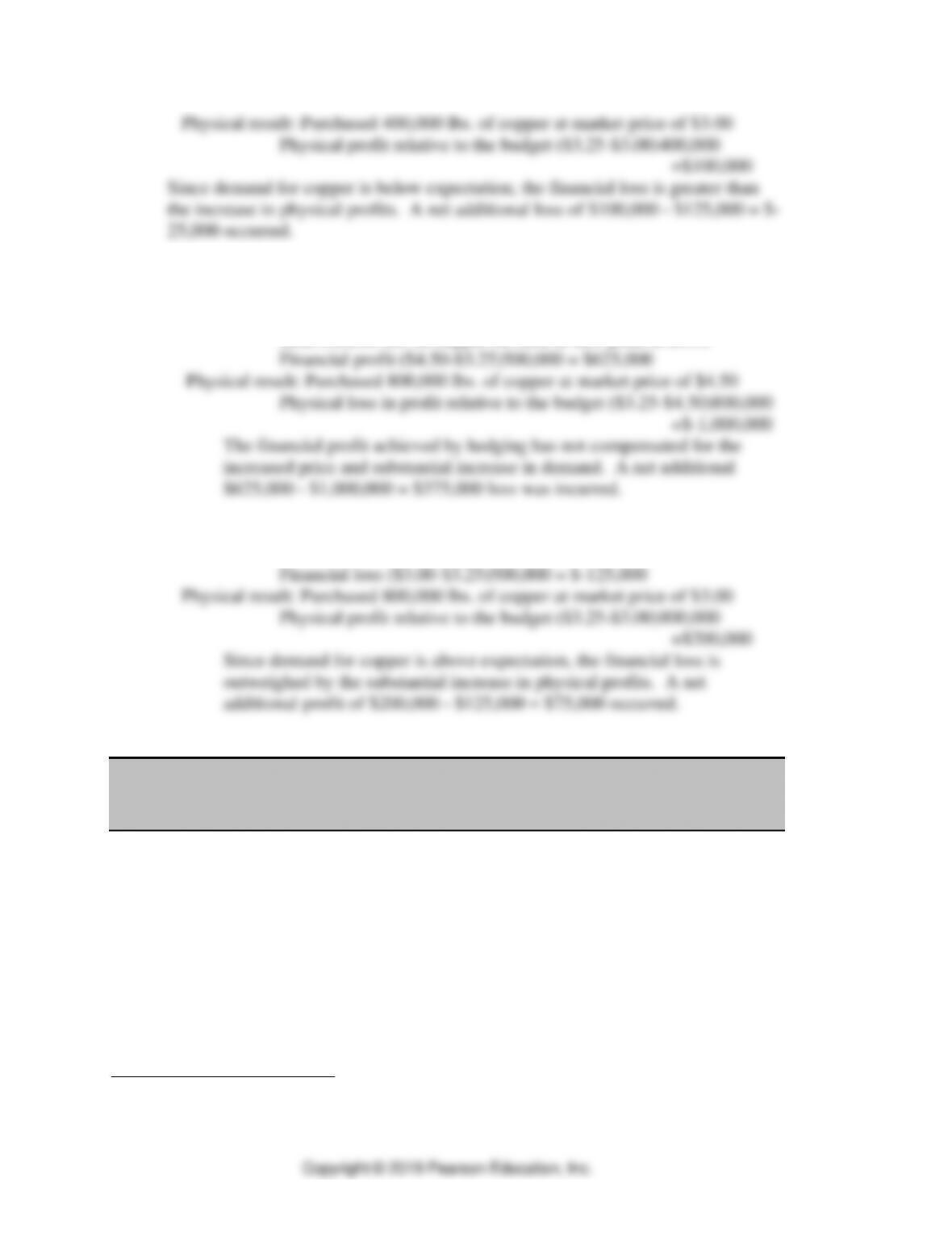
14. Eastmark continued
a. The firm has just lost a key client’s business and only purchases 400,000 lbs. of
copper.
i. Financial result: Paid $3.25 for 500,000 lbs. of copper on futures contract
ii. Financial result: Paid $3.25 for 500,000 lbs. of copper on futures contract
Sold 500,000 lbs. of copper for cash at new price at $3.00
Financial loss ($3.00-$3.25)500,000 = $-125,000
⚫ PART 3 ⚫ Managing Supply Chains
14–12
b. The firm has just gained a new client’s business and purchases 800,000 lbs. of
copper.
i. Financial result: Paid $3.25 for 500,000 lbs. of copper on futures contract
Sold 500,000 lbs. of copper for cash at new price at $4.50
ii. Financial result: Paid $3.25 for 500,000 lbs. of copper on futures contract
Sold 500,000 lbs. of copper for cash at new price at $3.00
CASE: WOLF MOTORS *
A. Synopsis
Wolf Motors has just expanded its network of auto dealerships to include its first
auto supermarket where three different makes of cars are sold at the same facility.
John Wolf, the president and owner of the dealership, has identified three factors
that have contributed to the success of the dealerships: volume, “one price-lowest
price” concept of pricing, and after-the-sale service to the cars sold. Focusing on the
service aspect, three components are critical to providing quality after-the-sale
service: well-trained technicians, the latest equipment technologies, and an adequate
supply of service parts and materials. Currently each dealership is responsible for
* This case was prepared by Dr. Brooke Saladin, Wake Forest University, as a basis for classroom
discussion.

Supply Chain Integration ⚫ CHAPTER 14 ⚫
14–13
ordering and managing its inventory of parts and service materials. The recent
growth has brought with it both space and financial resource constraints. John is
now wondering what, if anything, can be done with respect to the purchasing of
service parts and materials that would help address some of these concerns.
B. Purpose
This case provides students with the opportunity to investigate the supplier
relationship process of an organization in the service sector. Students begin to see
that the effective management of materials is not only essential in manufacturing
environments but is also critical in supporting the delivery of quality services.
Students are confronted by a number of issues as they are asked to recommend a
suitable structure for the supplier relationship process. Included among them are the
following:
1. Given the growth in the number of dealerships in the network, should the
supplier relationship process be centralized to take advantage of certain
economies of scale, or should it remain decentralized in each separate
dealership?
2. Given the different categories of service parts that are purchased, supplier
management issues are raised. Some parts may be more appropriately purchased
through single-source contracting, whereas others may be competitively bid on
by multiple suppliers. Bid awards don’t necessarily have to be awarded on the
basis of low cost alone. Also some items may be grouped and purchased from
the same supplier using blanket orders.
3. Limited space for inventory storage and limited investment dollars complicate
the issues. Fast, reliable service in repairing and servicing cars is a key factor in
the success of the dealership, but space and dollars limit service part availability
to some extent.
4. Finally, students have the opportunity to conceptually bring into play basic
inventory management concepts such as an ABC analysis to help determine
appropriate levels of inventory investment and inventory stocking policies. This
case can be used as a lead–in to Chapter 9, “Supply Chain Inventory
Management.”
C. Analysis
The analysis of this case can be accomplished in three logical steps. Students should
first address the issue of restructuring the supplier relationship process. Then the
inherent policies and procedures to carry out the purchasing processes can be
addressed, followed by an analysis of specific inventory management issues that
help lead into Chapter 9, “Supply Chain Inventory Management.”
Major factors to consider in addressing these steps include:
❑
Currently each individual dealership handles its own purchase and management
of service parts and materials.
⚫ PART 3 ⚫ Managing Supply Chains
14–14
❑
Wolf Motors is trying to reduce the total operating costs in order to compete
effectively in a very price competitive market with its “one price–lowest price”
strategy, while at the same time it needs to maintain a high level of service.
High service levels have traditionally been linked to high levels of inventory of
spare parts.
heat affects the air-conditioning, and rain affects the wipers.
1. Structural Issues: Students should first address the structural issues that face
Wolf Motors pertaining to the purchase of parts and materials. These issues
include two categories of decisions: (1) centralized purchasing versus continuing
a decentralized model of letting each dealership purchase and manage its own
inventories and (2) the responsibility relationships purchasing should maintain
with inventory management and control, including the distribution of parts for
service and over-the-counter sales.
Supply Chain Integration ⚫ CHAPTER 14 ⚫
14–15
2. Policies and Procedures: After the structural issues have been discussed,
students should consider alternative purchasing options that are available for
procuring parts. Given that the parts and materials being purchased differ quite a
bit with respect to availability, usage, costs, and delivery lead time, the policies
and procedures used to order various parts may be different. Alternative policies
that may be used include:
❑
Competitive bidding
Of course, these approaches are not mutually exclusive and may be combined
for certain categories of parts. Students should discuss how each of these
alternatives may be used for different groups of parts and materials. Going out
for competitive bids would be most appropriate for “commodity” type items that
are readily available from a number of vendors. Given that other aspects of the
service, such as reliability and dependability, are comparable, then a competitive
bid will help reduce purchase costs. Where the quality of the parts and/or service
provided differs, then a single-source contract may be warranted. This should
lead to a partnership arrangement that is beneficial to both parties.
3. Inventory Management Issues: The financial resource and space constraint
issues brought out in the case provide the opportunity to discuss the close
relationship and necessary integration that purchasing must have with inventory
⚫ PART 3 ⚫ Managing Supply Chains
14–16
❑
You can discuss the different costs incurred in ordering and carrying
inventory to reinforce the trade-offs in these costs discussed in Chapter 10,
“Supply Chain Design.”
❑
You can bring out the issue of total investment in inventory over time to
open the door for a discussion of the ABC analysis in Chapter 9, “Supply
Chain Inventory Management.”
D. Recommendations
How the case is used will determine the level of detail you should expect with
respect to any recommendations students may make. When used as an in-class
exercise without any prior preparation by the students, the focus of the case should
be on discussing the issues and recognizing the trade-offs that need to be made in
the decisions. If given more time to read and analyze the case, typical
recommendations to expect include:
1. Some form of centralization of the purchasing function
2. Development of partnership agreements for “key” parts that perhaps may lead to
single sourcing
3. The use of blanket orders to reduce ordering costs and to limit the number of
suppliers
4. Open-ended ordering agreements, especially in the “commodity” type materials
that can be sourced locally to reduce lead times and minimize inventory
investment
5. Perhaps the establishment of a central warehouse facility to reduce overall space
requirements while maintaining parts availability in a timely manner
6. Conducting an analysis of inventory cost trade-offs to minimize total costs of
inventory policies
E. Teaching Suggestions
This case can be used as either an in-class “cold–call” exercise or an overnight
reading and analysis exercise. In either case the class discussion flows well when
the instructor follows the order of the discussion questions at the end of the case.
The level of detail necessary to make this a good decision case is not present. The
case was designed to act as a vehicle to introduce the issues that pertain to the
supplier relationship process and to show students that the issues are similar in both

Supply Chain Integration ⚫ CHAPTER 14 ⚫
14–17
services and manufacturing. Therefore, it is best to begin the discussion by first
focusing on how the supplier relationship process should be organized. Then focus
the students on specific policies and procedures that Wolf may implement for
different categories of parts. Finally, if time permits, you can begin to introduce
some inventory management issues and show how the inventory function interacts
with purchasing.