Supply Chain Logistic Networks ⚫ CHAPTER 13 ⚫
Dummy location and is therefore is not used. Shipments to the Dummy location from F2
and F3 represent unused capacity.
Total Cost: F2-W1= 45,000($2) = $90,000
19. Thor International Company (part 2)
a. Once again using the Transportation Method (Location) module in POMS for
Windows, we get the optimal solution shown in the output that follows.
Module/submodel: Transportation Method (Location)
Problem title: Thor International
Objective: Minimize
Original Data
W1 W2 W3 W4 W5 Dummy
————————————————————————-
F1 2 3 3 2 6 0
Capacity
———————
F1 50000
F2 80000
F3 80000
DEMAND
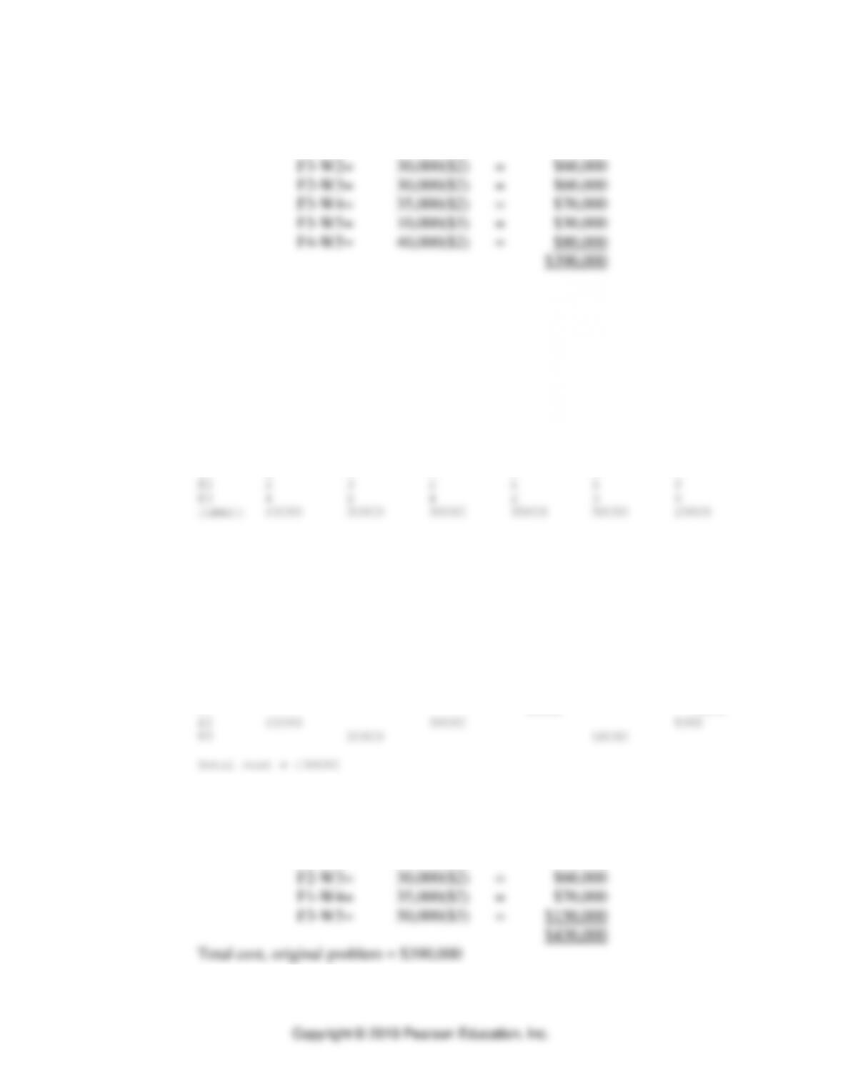
Shipments
W1 W2 W3 W4 W5 Dummy
————————————————————————-
F1 35000 15000
With this solution, the total cost of the revised problem is greater than the total cost in
problem 18. Thus, the logistic manager should get a budget increase.
Total Cost: F2-W1= 45,000($2) = $90,000
F3-W2= 30,000($2) = $60,000
⚫ PART 3 ⚫ Managing Supply Chains
b. The logistics manager should receive a budget increase of ($430,000 – $390,000) =
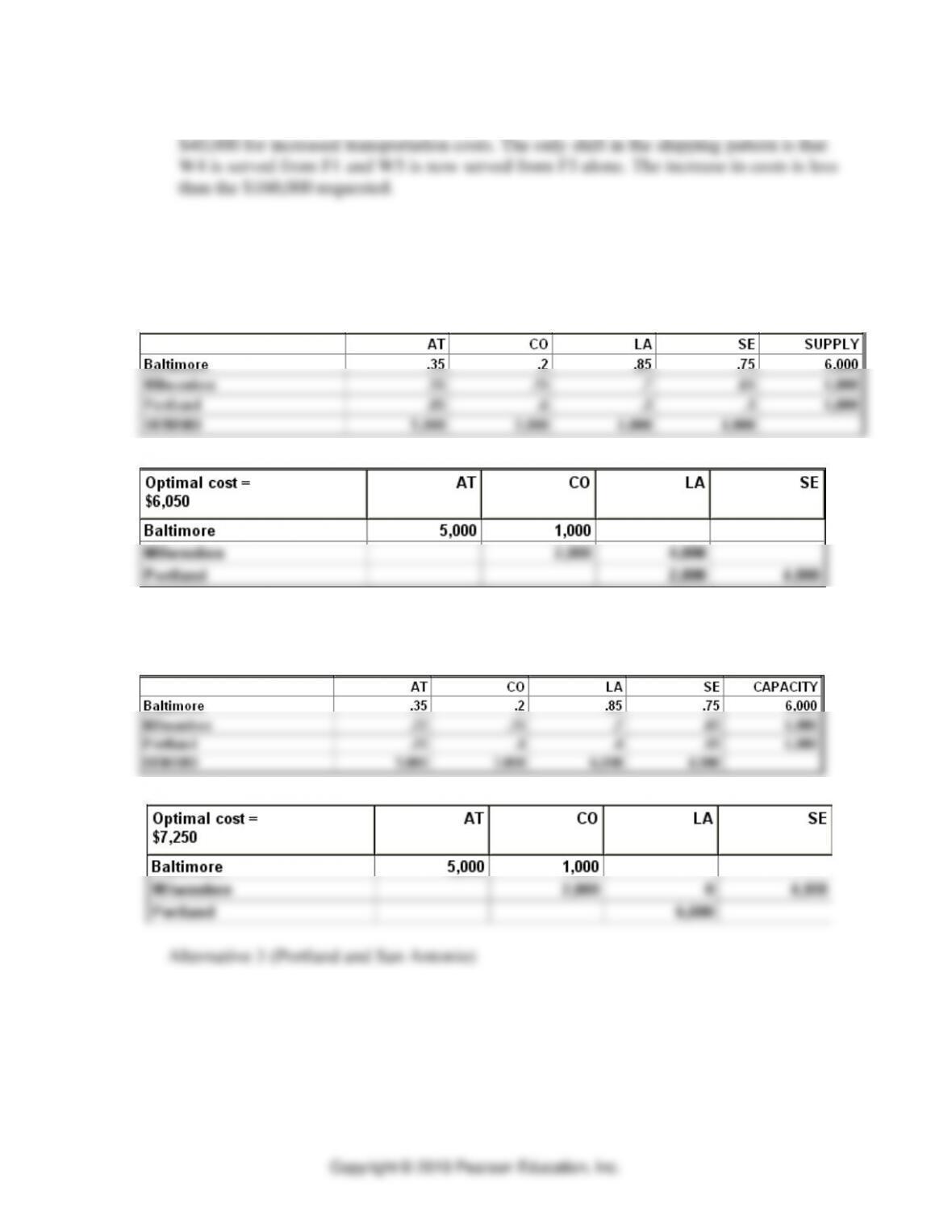
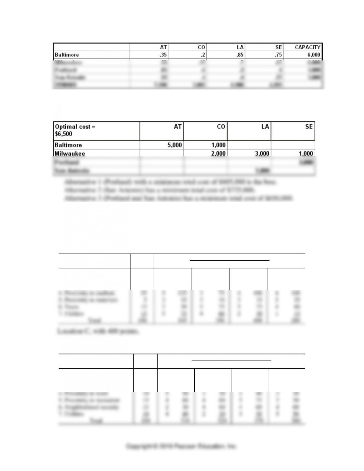
20. Chambers Corporation
Using Transportation Method (Location) module in POMS for Windows
Alternative 1 (Portland)
Data Screen
Solution Screen
Alternative 2 (San Antonio)
Data Screen
Solution Screen
Data Screen
Supply Chain Logistic Networks ⚫ CHAPTER 13 ⚫
Solution Screen
A Systematic Location Selection Process
21. Preference matrix location for A, B, C, or D
Factor
Factor Score for Each Location
Location Factor
Weight
A
B
C
D
1. Labor climate
5
5
25
4
20
3
15
5
25
2. Quality of life
30
2
60
3
90
5
150
1
30
3. Transportation system
5
3
15
4
20
3
15
5
25
4. Proximity to markets
25
5
125
3
75
4
100
4
100
5. Proximity to materials
5
3
15
2
10
3
15
5
25
6. Taxes
15
2
30
5
75
5
75
4
60
7. Utilities
15
5
75
4
60
2
30
1
15
Total
100
345
350
400
280
22. John and Jane Darling
Factor
Factor Score for Each Location
Location Factor
Weight
A
B
C
D
1. Rent
25
3
75
1
25
2
50
5
125
2. Quality of life
20
2
40
5
100
5
100
4
80
3. Schools
5
3
15
5
25
3
15
1
5
4. Proximity to work
10
5
50
3
30
4
40
3
30
5. Proximity to recreation
15
4
60
4
60
5
75
2
30
6. Neighborhood security
15
2
30
4
60
4
60
4
60
7. Utilities
10
4
40
2
20
3
30
5
50
Total
100
310
320
370
380
⚫ PART 3 ⚫ Managing Supply Chains
Copyright © 2019 Pearson Education, Inc.
Location D, the in-laws’ downstairs apartment, is indicated by the highest score. This points
out a criticism of the technique: the Darlings did not include or give weight to a relevant
factor.
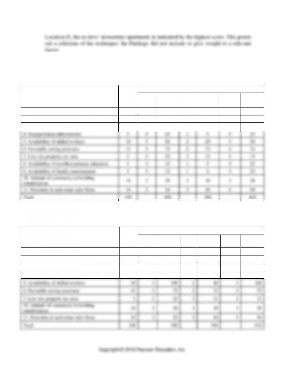
23. Wagner Remodelers Inc.
a. As seen in the following calculation table, Royce has the highest Total Weighted
Factor score and is thereby considered the superior location
Location Factor
Factor
Weight
Factor Score for Each City
Coptic
Weighted
Factor
Sparta
Weighted
Factor
Royce
Weighted
Factor
1. Proximity to run-down housing stock
15
3
45
5
75
1
15
2. Community population size
15
3
45
5
75
5
75
3. Proximity to the sources of building materials
5
5
25
5
25
5
25
4. Transportation infrastructure
5
5
25
1
5
5
25
5. Availability of skilled workers
10
5
50
2
20
5
50
6. Favorable zoning processes
15
5
75
5
75
5
75
7. Low city property tax rates
5
5
25
3
15
3
15
8. Availability of excellent primary education
5
3
15
1
5
5
25
9. Availability of family entertainment
5
3
15
1
5
5
25
10. Attitude of community to building
rehabilitation
10
2
20
3
30
3
30
11. Proximity to real estate sales firms
10
2
20
5
50
5
50
Total
100
360
380
410
b. The superior location did not change; as seen in the following table, Royce still has the
highest Total Weighted Factor score
Location Factor
Factor
Weight
Factor Score for Each City
Coptic
Weighted
Factor
Sparta
Weighted
Factor
Royce
Weighted
Factor
1. Proximity to run-down housing stock
15
3
45
5
75
1
15
2. Community population size
15
3
45
5
75
5
75
3. Proximity to the sources of building materials
5
5
25
5
25
5
25
4. Transportation infrastructure
5
5
25
1
5
5
25
5. Availability of skilled workers
20
5
100
2
40
5
100
6. Favorable zoning processes
15
5
75
5
75
5
75
7. Low city property tax rates
5
5
25
3
15
3
15
10. Attitude of community to building
rehabilitation
10
2
20
3
30
3
30
11. Proximity to real estate sales firms
10
2
20
5
50
5
50
Total
100
380
390
410
Supply Chain Logistic Networks ⚫ CHAPTER 13 ⚫
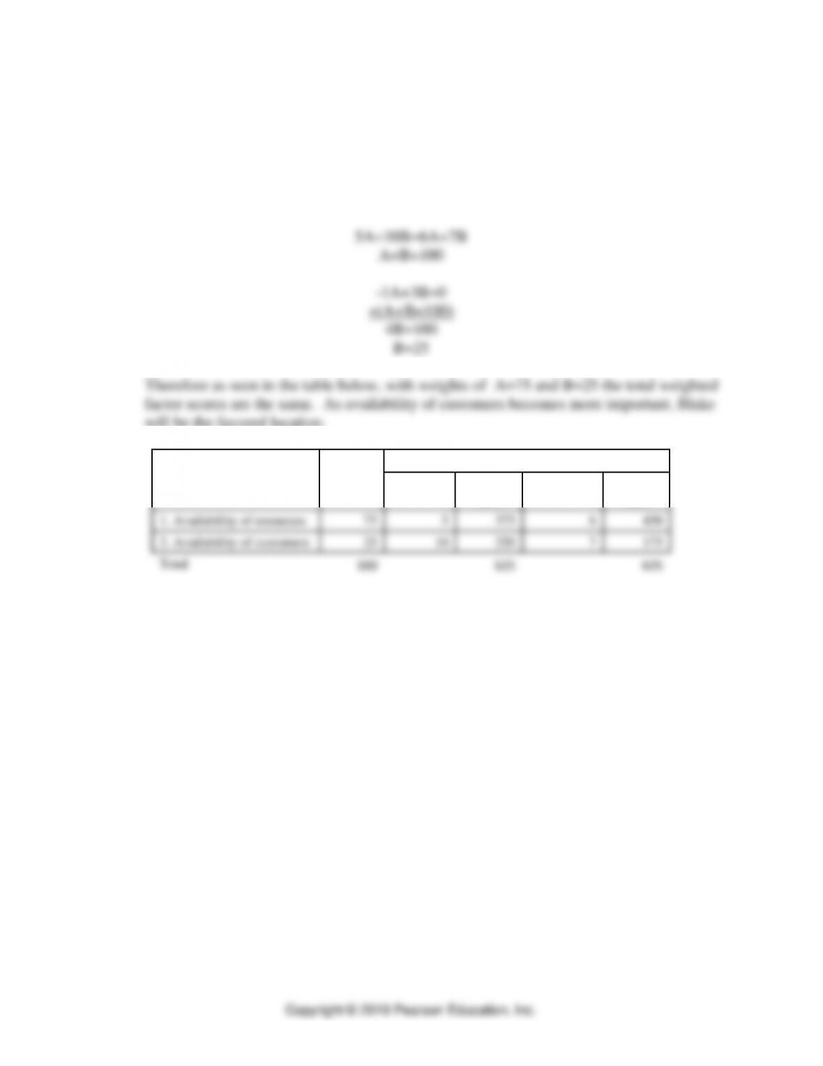
24. Silky Industries
Solving this problem as 2 equations in 2 unknowns with A representing “availability of
resources” and B representing “availability of customers”:
will be the favored location.
Location Factor
Factor
Weight
Factor Score for Each City
Blake
Weighted
Factor
Irmo
Weighted
Factor
1. Availability of resources
75
5
375
6
450
2. Availability of customers
25
10
250
7
175
Total
100
625
625
⚫ PART 3 ⚫ Managing Supply Chains
CASE: R. U. Reddie for Location
A. Overview
Rhonda Reddie, owner and CEO of a company that manufactures wardrobes for stuffed animals,
is faced with the prospect of sizeable demand increases in the near future with insufficient
capacity to take advantage of it. Expanding capacity at her existing plants is not an option for
various reasons. Consequently, she must decide if it is a good idea to increase capacity by
purchasing a new plant. If the answer is yes, then she must decide where the plant should be
located. The two options she would consider are St. Louis and Denver.
B. Purpose
This case was written to provide the student with enough data to analyze the decisions Reddie
must make, using tools such as the transportation method and net present values. Students learn
where the cost figures come from that are used in the cash flow analysis and net present value
calculations. In this case, the location decision will affect the cost of goods sold because of
differing cost factors at each location which affect the distribution patterns in the supply
network. In addition, the capital costs of the plant and equipment differ by location, as does the
cost of the land. Consequently, the location decision affects annual operating costs, the extent of
the capital investment, and hence the financial results as represented by the net present value of
the investment. Instructors can use the case to demonstrate the cross-functional aspects of these
major decisions in practice.
C. Transportation Models
Appendix A contains the linear programming models for Denver and St. Louis in matrix form.
The models determine the optimal shipping pattern if Denver or St. Louis are the chosen
locations. The objective function value is the optimal cost of goods sold for the entire network of
plants with a given option for the new fourth plant. The demand data are the “most likely”
estimates given in the case. Students will have to determine the objective function coefficients,
which consist of the variable production cost per unit at a plant plus the transportation cost to
ship one unit from the plant to one of the destinations in the supply chain. The distribution cost is
$0.0005: The actual cost to ship to another destination will depend on the number of miles the
unit must be shipped. For example, the cost to produce one unit in Cleveland and ship it to
Boston is $3.00 + $0.0005 (650 miles) = $3.325.
Supply Chain Logistic Networks ⚫ CHAPTER 13 ⚫
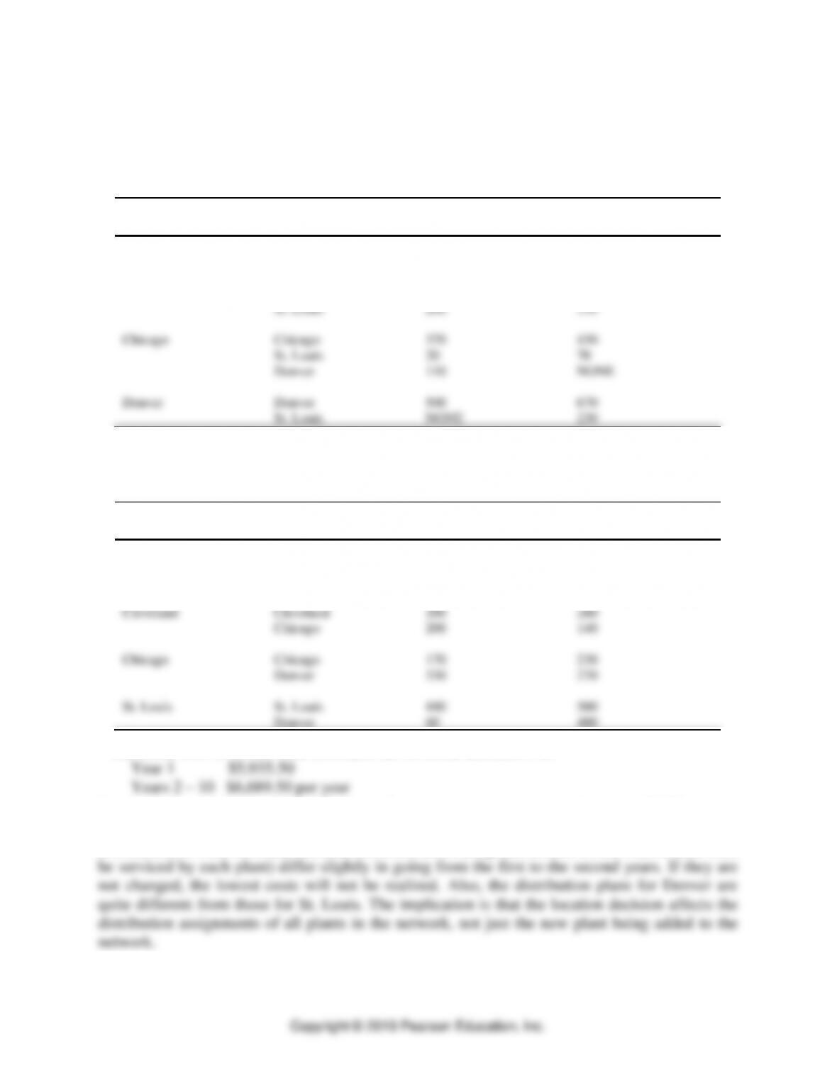
D. Optimal Distribution Plans for each Location
There are actually two distribution plans for each location: One for year 1 and another for years 2
and beyond. Appendix A contains the computer output from POM for Windows for the two
options. The tables below provide the optimal distribution plans and costs.
Denver
From
To
Year 1
Years 2 to 10
Boston
Boston
80
140
St. Louis
220
60
Cleveland
Cleveland
200
260
St. Louis
200
140
Chicago
Chicago
370
430
St. Louis
20
70
Denver
110
NONE
Denver
Denver
500
670
St. Louis
NONE
230
The Total Cost of Goods Sold ($000) for the Denver alternative is:
Year 1 $5,790
Years 2 – 10 $6,606.25 per year
St. Louis
From
To
Year 1
Years 2 to 10
Boston
Boston
80
140
Denver
220
NONE
Chicago
NONE
60
Cleveland
Cleveland
200
260
Chicago
200
140
Chicago
Chicago
170
230
Denver
330
270
St. Louis
St. Louis
440
500
Denver
60
400
The Total Cost of Goods Sold ($000)for the St. Louis alternative is:
Several things can be noted at this stage. First, on the basis of variable costs (COGS) alone,
Denver seems to be the better choice. However, as we shall see later, other financial
considerations must be made. Second, the distribution assignments (i.e., which warehouses must
⚫ PART 3 ⚫ Managing Supply Chains
E. Net Present Value
One important measure of the viability of a location decision involving capital outlays is the use
of a net present value (NPV) criterion. However, in this case we must compute incremental cash
flows because the new plant is to be used as a member of an existing network of plants. The only
measures of cash flow we get here is the total system COGS with and without the new
investment. The case gives the COGS for a Status Quo (without the new plants) solution so that
these incremental costs attributable to the new investment can be computed. For example, the
Denver alternative will generate the following incremental COGS ($000):
Denver Status Quo Incremental COGS
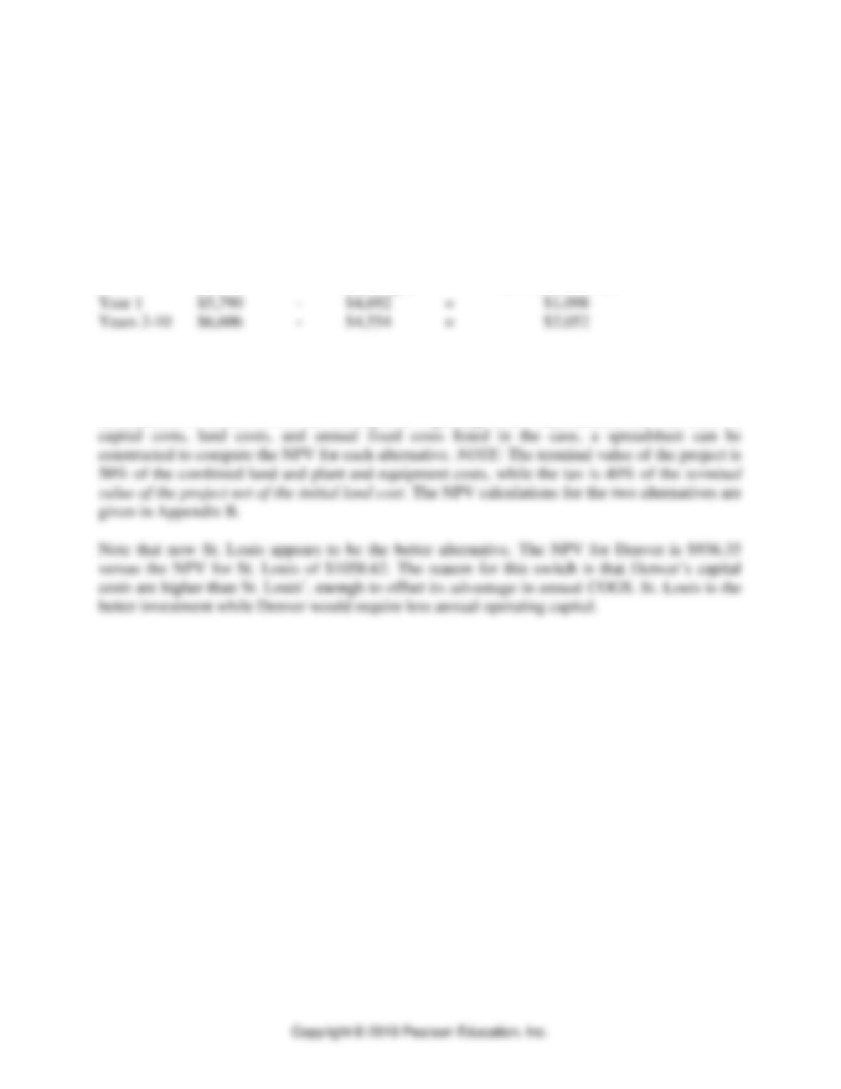
The revenue flows due to the addition of a new plant are the same regardless of the location. In
year 1, 400 (000) additional units can be sold at a price of $8 per unit, for an incremental
addition of $3,200. In years 2 and beyond, 700 (000) additional units will generate $5,600 in
incremental revenues. Given the assumptions regarding taxes, depreciation, and the data on
Supply Chain Logistic Networks ⚫ CHAPTER 13 ⚫
F. Conclusions
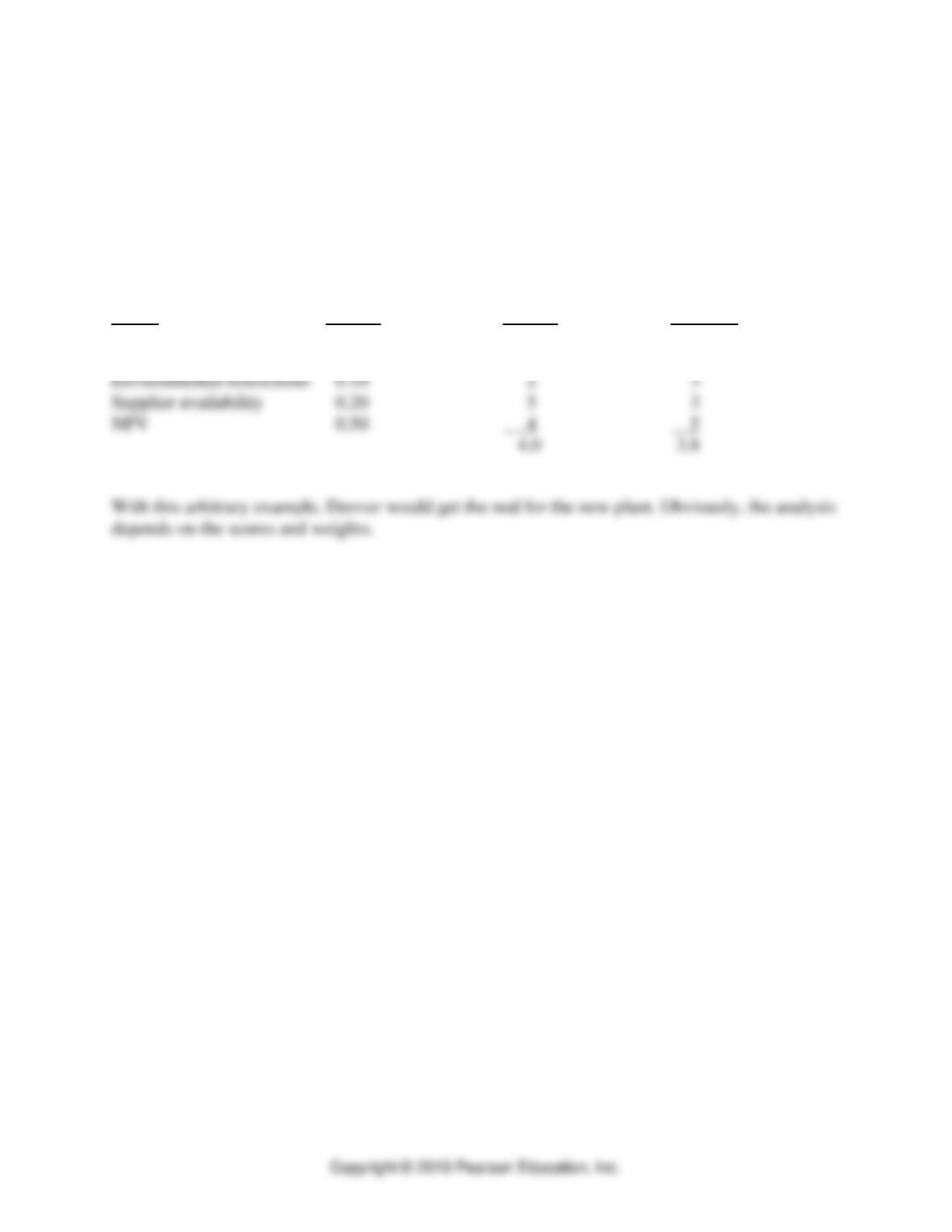
The case raised some non-quantitative factors in this decision. The instructor should press the
students as to how they would reconcile these factors, particularly since two of the three favor
Denver. One way to rationalize the decision is to use a preference matrix where each alternative
can be scored subjectively across all the major criteria. For example, using the base case in
which St. Louis had the better NPV, we might have the following matrix where a score of 5 is
excellent and a 1 is poor:
Factor Weight Denver St. Louis
Workforce availability 0.20 4 2
⚫ PART 3 ⚫ Managing Supply Chains
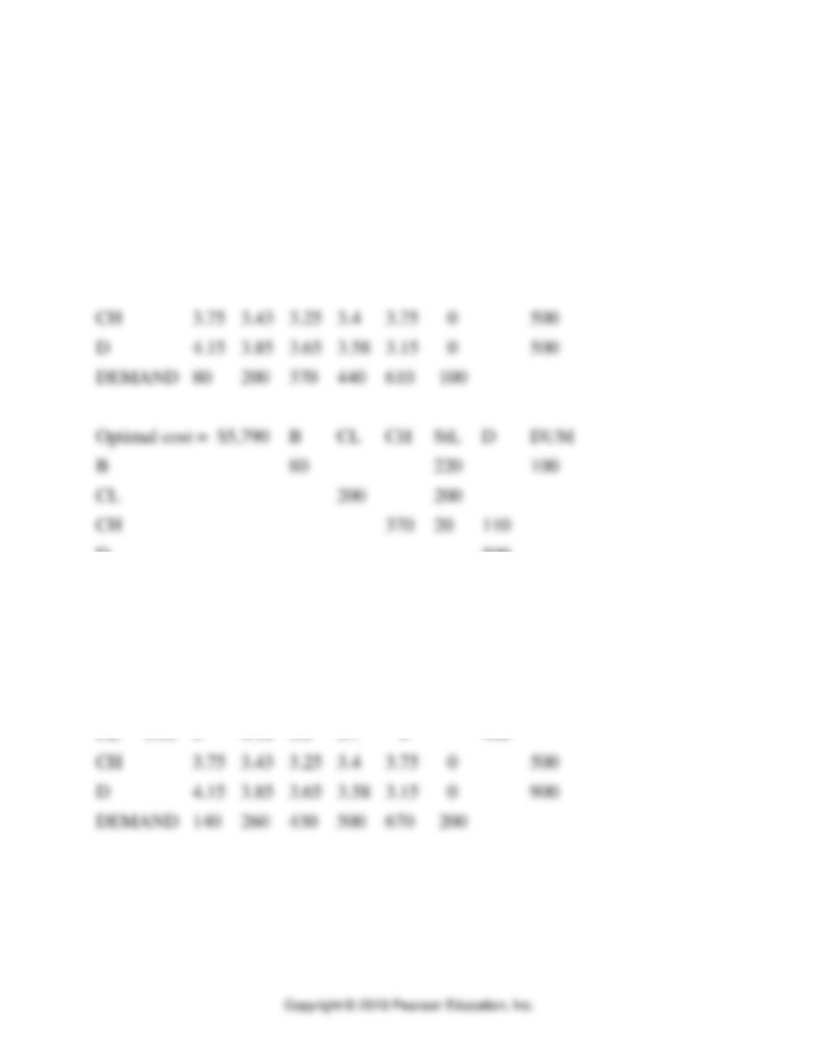
Appendix A
Denver Year 1
B CL CH StL D DUM SUPPLY
B 3.8 4.13 4.3 4.4 4.8 0 400
CL 3.33 3 3.18 3.3 3.7 0 400
D 500
Denver Years 2 – 10
B CL CH StL D DUM SUPPLY
B 3.8 4.13 4.3 4.4 4.8 0 400
CL 3.33 3 3.18 3.3 3.7 0 400
Supply Chain Logistic Networks ⚫ CHAPTER 13 ⚫
Optimal cost = $6,606.25 B CL CH StL D DUM
B 140 60 200
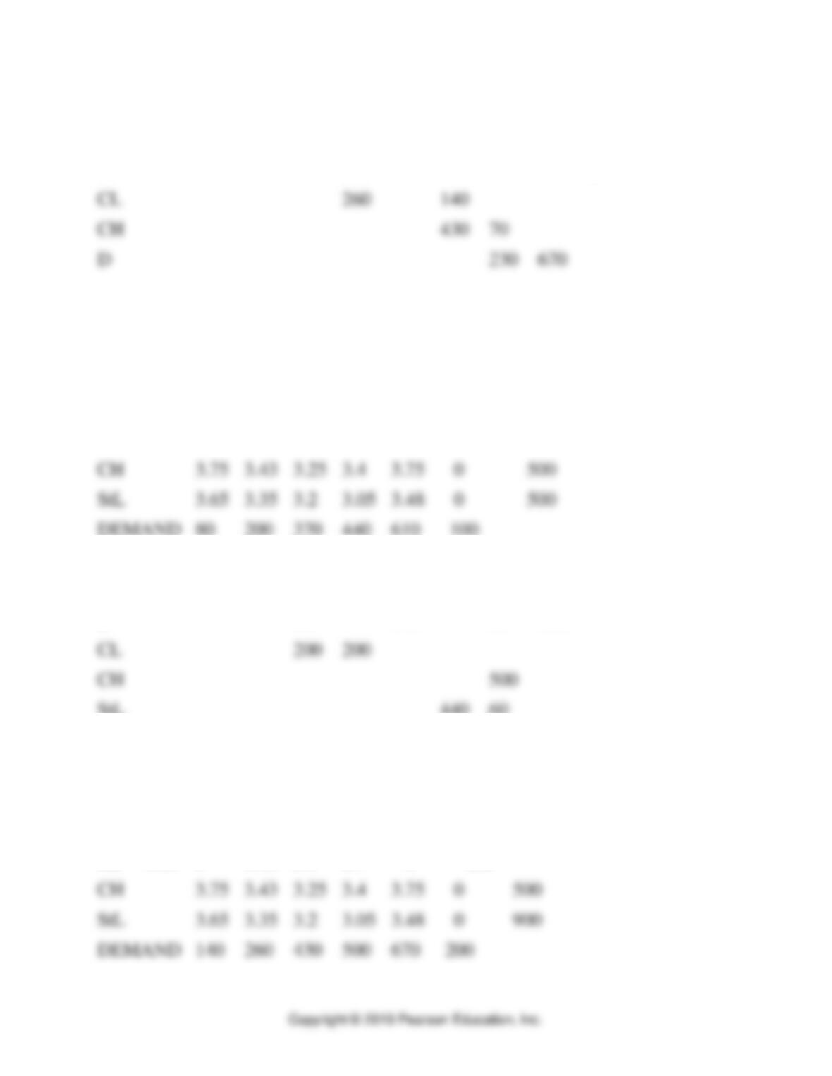
St Louis Year 1
B CL CH StL D DUM SUPPLY
B 3.8 4.13 4.3 4.4 4.8 0 400
CL 3.33 3 3.18 3.3 3.7 0 400
Optimal cost = $5,935.5 B CL CH StL D DUM
B 80 170 50 100
StL 440 60
St Louis Years 2 – 10
B CL CH StL D DUM SUPPLY
B 3.8 4.13 4.3 4.4 4.8 0 400
CL 3.33 3 3.18 3.3 3.7 0 400
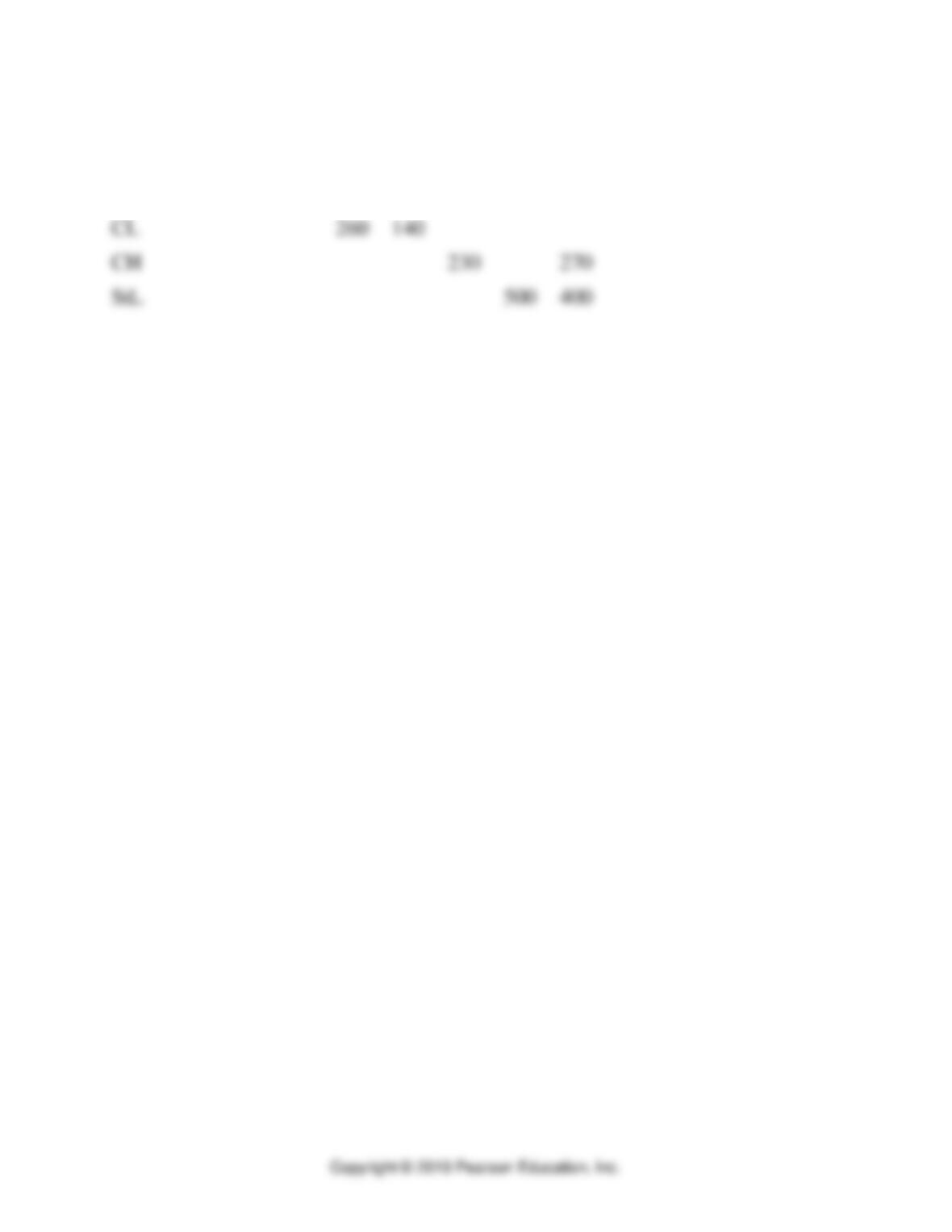
⚫ PART 3 ⚫ Managing Supply Chains
Optimal cost = $6,689.5 B CL CH StL D DUM
B 140 60 200
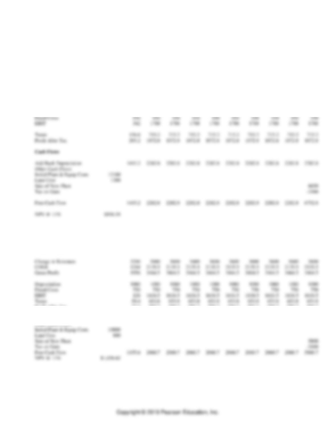
Appendix B
Denver Location NPV⎯Most Likely
Denver
0
1
2
3
4
5
6
7
8
9
10
Profit or Loss
Change in Revenues
3200
5600
5600
5600
5600
5600
5600
5600
5600
5600
COGS
1098
2052
2052
2052
2052
2052
2052
2052
2052
2052
Gross Profit
2102
3548
3548
3548
3548
3548
3548
3548
3548
3548
Depreciation
1210
1210
1210
1210
1210
1210
1210
1210
1210
1210
Fixed Costs
550
550
550
550
550
550
550
550
550
550
EBIT
342
1788
1788
1788
1788
1788
1788
1788
1788
1788
Taxes
136.8
715.2
715.2
715.2
715.2
715.2
715.2
715.2
715.2
715.2
Profit After Tax
205.2
1072.8
1072.8
1072.8
1072.8
1072.8
1072.8
1072.8
1072.8
1072.8
Cash Flows
Add Back Depreciation
1415.2
2282.8
2282.8
2282.8
2282.8
2282.8
2282.8
2282.8
2282.8
2282.8
Other Cash Flows
Initial Plant & Equip Costs
12100
Land Cost
1200
Sale of New Plant
6650
Tax on Gain
-2180
Free Cash Flow
1415.2
2282.8
2282.8
2282.8
2282.8
2282.8
2282.8
2282.8
2282.8
6752.8
NPV @ 11%
$936.35
St. Louis Location NPV⎯Most Likely
St. Louis
0
1
2
3
4
5
6
7
8
9
10
Profit or Loss
Change in Revenues
3200
5600
5600
5600
5600
5600
5600
5600
5600
5600
COGS
1244
2135.5
2135.5
2135.5
2135.5
2135.5
2135.5
2135.5
2135.5
2135.5
Gross Profit
1956
3464.5
3464.5
3464.5
3464.5
3464.5
3464.5
3464.5
3464.5
3464.5
Depreciation
1080
1080
1080
1080
1080
1080
1080
1080
1080
1080
Fixed Costs
750
750
750
750
750
750
750
750
750
750
EBIT
126
1634.5
1634.5
1634.5
1634.5
1634.5
1634.5
1634.5
1634.5
1634.5
Taxes
50.4
653.8
653.8
653.8
653.8
653.8
653.8
653.8
653.8
653.8
Profit After Tax
75.6
980.7
980.7
980.7
980.7
980.7
980.7
980.7
980.7
980.7
Cash Flows
Add Back Depreciation
1155.6
2060.7
2060.7
2060.7
2060.7
2060.7
2060.7
2060.7
2060.7
2060.7
Other Cash Flows
Initial Plant & Equip Costs
10800
Land Cost
800
Sale of New Plant
5800
Tax on Gain
-2000
Free Cash Flow
1155.6
2060.7
2060.7
2060.7
2060.7
2060.7
2060.7
2060.7
2060.7
5860.7
NPV @ 11%
$1,058.62