Chapter
13
Supply Chain Logistic Networks
DISCUSSION QUESTIONS
1. Answers depend on the specific organizations and industries selected by the teams. Some
expected tendencies for manufacturers are:
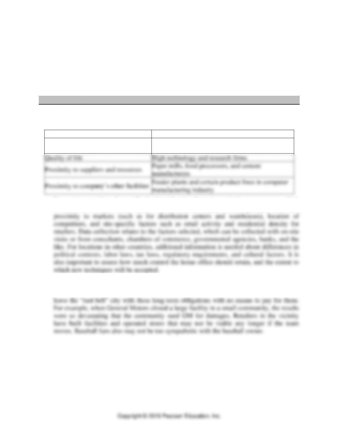
Favorable labor climate
Textiles, furniture, consumer electronics
Proximity to markets
Paper, plastic pipe, cars, heavy metals, and food
processing
Quality of life
High technology and research firms
Proximity to suppliers and resources
Paper mills, food processors, and cement
manufacturers
Proximity to company’s other facilities
Feeder plants and certain product lines in computer
manufacturing industry
For service providers, the usually dominant location factor is proximity to customers, which
is related to revenues. Other factors that also can be crucial are transportation costs and
2. The “rust belt” city has made long-term investments in the stadium, roads, zoning, and
planning to the benefit of the baseball team (an entertainment service). Relocation would
3. The firm would be well advised to consider both the current state of affairs and potential
future action required should the firm finalize this plant location decision. Once the plant is
purchased, the firm may take on responsibility for remediating previous plant-management
decisions.
Regarding the environmental impact of current practices, the firm should consider such
aspects as (1) the plant’s current carbon footprint and the costs to reduce, (2) the carbon
⚫ PART 3 ⚫ Managing Supply Chains
footprint of suppliers that may be used should this location be selected, (3) overall plant
Supply Chain Logistic Networks ⚫ CHAPTER 13 ⚫
PROBLEMS
Load-Distance Method
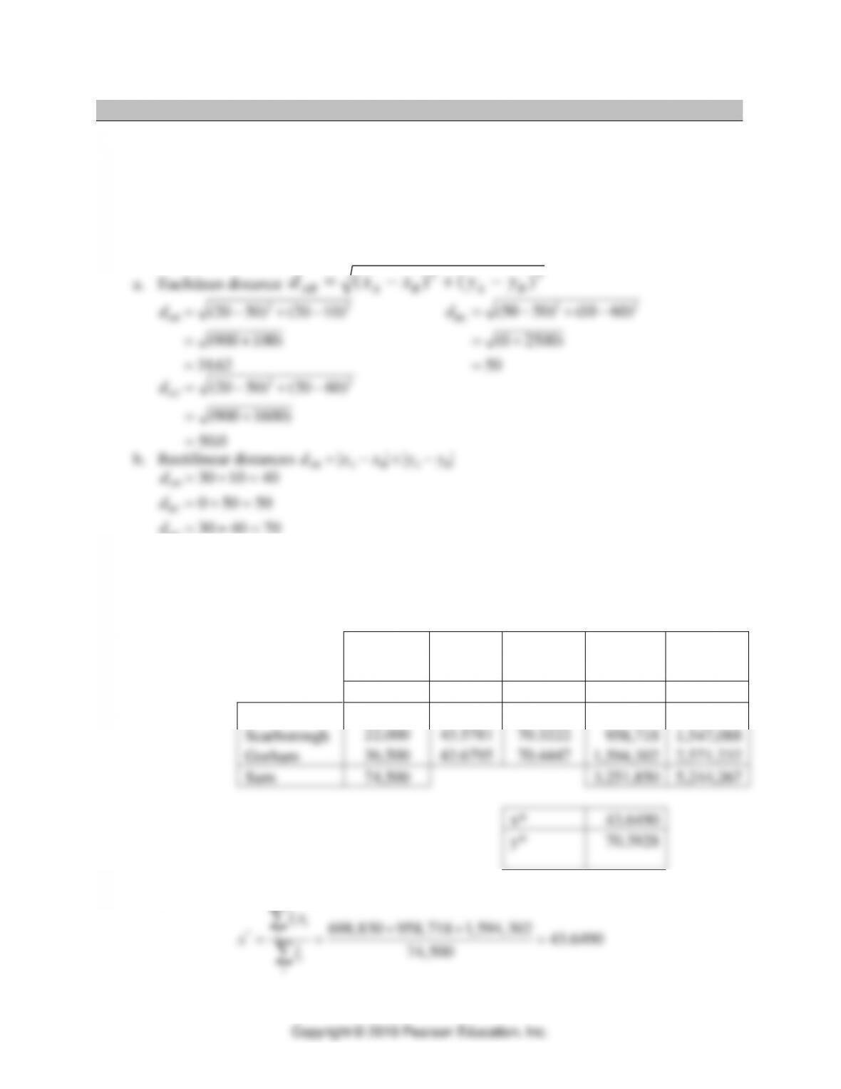
1. Distance between three points
Point A = (20, 20)
Point B = (50, 10)
Point C = (50, 60)
22 )()( BABAAB yyxxd −+−=
⚫ PART 3 ⚫ Managing Supply Chains
Copyright © 2019 Pearson Education, Inc.
*1,125,947 1,547, 088 2,571, 232 70.3928
74,500
ii
i
i
i
ly
yl
++
= = =
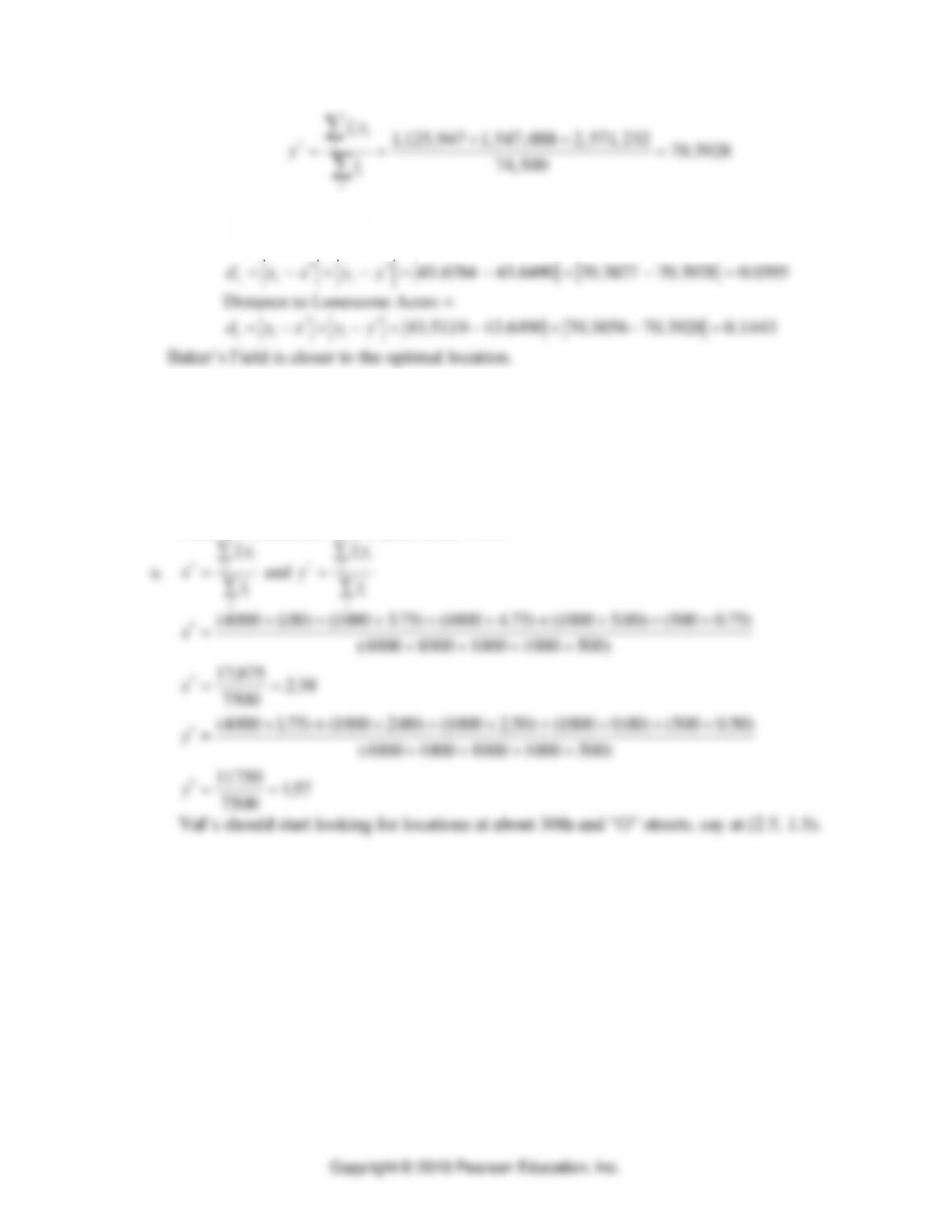
b. The rectilinear distance from the optimal location to the available land parcels are:
Distance to Baker’s Field =
0395.03928.703827.706490.436784.43
** =−+−=−+−= yyxxd iii
Distance to Lonesome Acres =
**
43.5119 43.6490 70.3856 70.3928 0.1443
i i i
d x x y y= − + − = − + − =
Baker’s Field is closer to the optimal location.
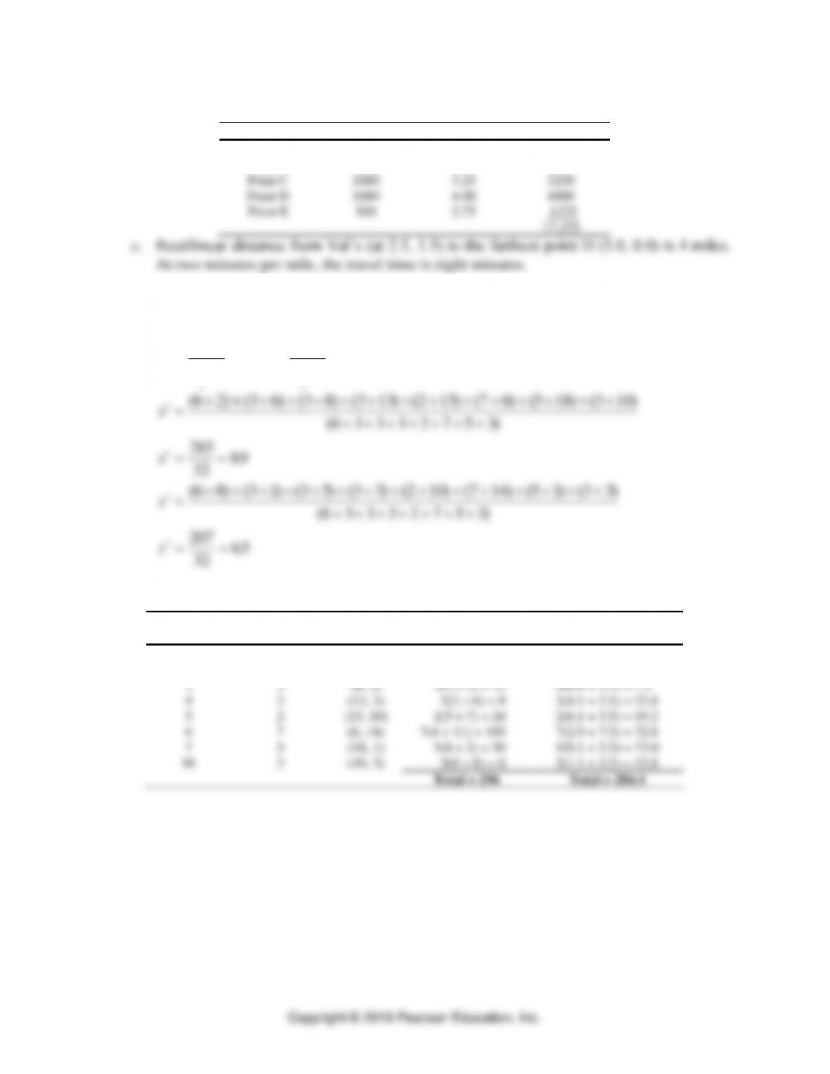
3. Val’s Pizza
Treating the southwest corner of the plot as the origin and estimating the coordinates,
Point A location (1.00, 1.75), demand = 4000
Point B location (3.75, 2.00), demand = 1000
Point C location (4.75, 2.50), demand = 1000
Point D location (5.00, 0.00), demand = 1000
Point E location (0.75, 0.50), demand = 500
l x
i i
i
*=
l y
i i
i
*=
Supply Chain Logistic Networks ⚫ CHAPTER 13 ⚫
b. Rectilinear load-distance score. Assuming Val’s location at (2.5, 1.5).
Location
Load
Distance
ld score
Point A
4000
1.75
7000
Point B
1000
1.75
1750
Point C
1000
3.25
3250
Point D
1000
4.00
4000
Point E
500
2.75
1375
17,375
c. Rectilinear distance from Val’s (at 2.5, 1.5) to the farthest point D (5.0, 0.0) is 4 miles.
At two minutes per mile, the travel time is eight minutes.
4. Davis, California, Post Office
a. Center of Gravity
x
l x
l
i i
i
i
i
*=
and
y
l y
l
i i
i
i
i
*=
x
x
y
y
*
*
*
*
.
.
=
( ) +
( ) +
( ) +
( ) +
( ) +
( ) +
( ) +
( )
+ + + + + + +
( )
= =
=
( ) +
( ) +
( ) +
( ) +
( ) +
( ) +
( ) +
( )
+ + + + + + +
( )
= =
6 2 3 6 3 8 3 13 215 7 6 5 18 310
6 3 3 3 2 7 5 3
285
32 8 9
6 8 3 1 3 5 3 3 2 10 714 5 1 3 3
6 3 3 3 2 7 5 3
207
32 65
b. Load distance scores
Mail Source
Point
Round Trips
per Day (l)
xy–
Coord
Load-distance to
M: (10, 3)
Load-distance to
CG: (8.9, 6.5)
1
6
(2, 8)
6(8 + 5) = 78
6(6.9 + 1.5) = 50.4
2
3
(6, 1)
3(4 + 2) = 18
3(2.9 + 5.5) = 25.2
3
3
(8, 5)
3(2 + 2) = 12
3(0.9 + 1.5) = 7.2
4
3
(13, 3)
3(3 + 0) = 9
3(4.1 + 3.5) = 22.8
5
2
(15, 10)
2(5 + 7) = 24
2(6.1 + 3.5) = 19.2
6
7
(6, 14)
7(4 + 11) = 105
7(2.9 + 7.5) = 72.8
7
5
(18, 1)
5(8 + 2) = 50
5(9.1 + 5.5) = 73.0
M
3
(10, 3)
3(0 + 0) = 0
3(1.1 + 3.5) = 13.8
Total = 296
Total = 284.4
⚫ PART 3 ⚫ Managing Supply Chains
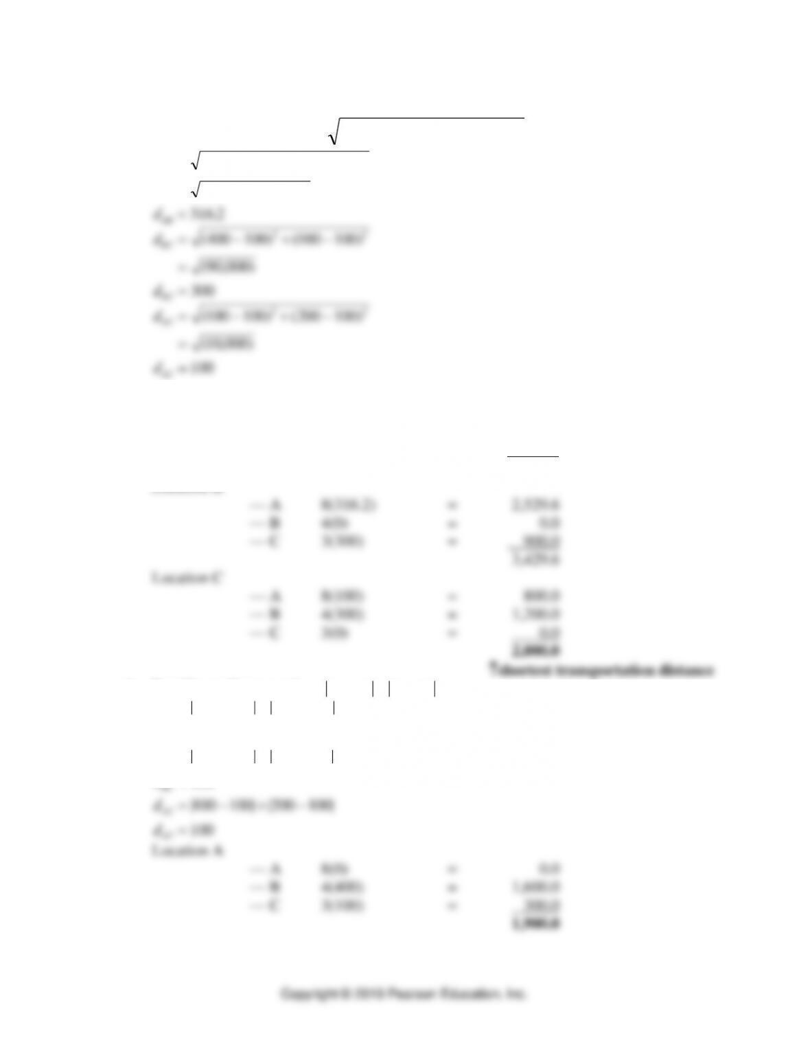
5. Rauschenberg Manufacturing
a. Euclidean distance
22 )()( BABAAB yyxxd −+−=
d
d
AB
AB
= − + −
= +
=
( ) ( )
( )
100 400 200 100
90 000 10 000
316 2
2 2
, ,
.
d
d
BC
BC
= − + −
=
=
( ) ( )
( )
400 100 100 100
90 000
300
2 2
,
d
d
AC
AC
= − + −
=
=
( ) ( )
( )
100 100 200 100
10 000
100
2 2
,
Location A
— A
8(0)
=
0.0
— B
4(316.2)
=
1,264.8
— C
3(100)
=
300.0
1,564.8
Location B
— A
8(316.2)
=
2,529.6
— B
4(0)
=
0.0
— C
3(300)
=
900.0
3,429.6
— A
8(100)
=
800.0
— B
4(300)
=
1,200.0
— C
3(0)
=
0.0
2,000.0
shortest transportation distance
b. Rectilinear distances
d x x y y
AB A B A B
= − + −
d
d
d
d
d
d
AB
AB
BC
BC
AC
AC
= − + −
=
= − + −
=
= − + −
=
100 400 200 100
400
400 100 100 100
300
100 100 200 100
100
— A
8(0)
=
0.0
— B
4(400)
=
1,600.0
— C
3(100)
=
300.0
1,900.0
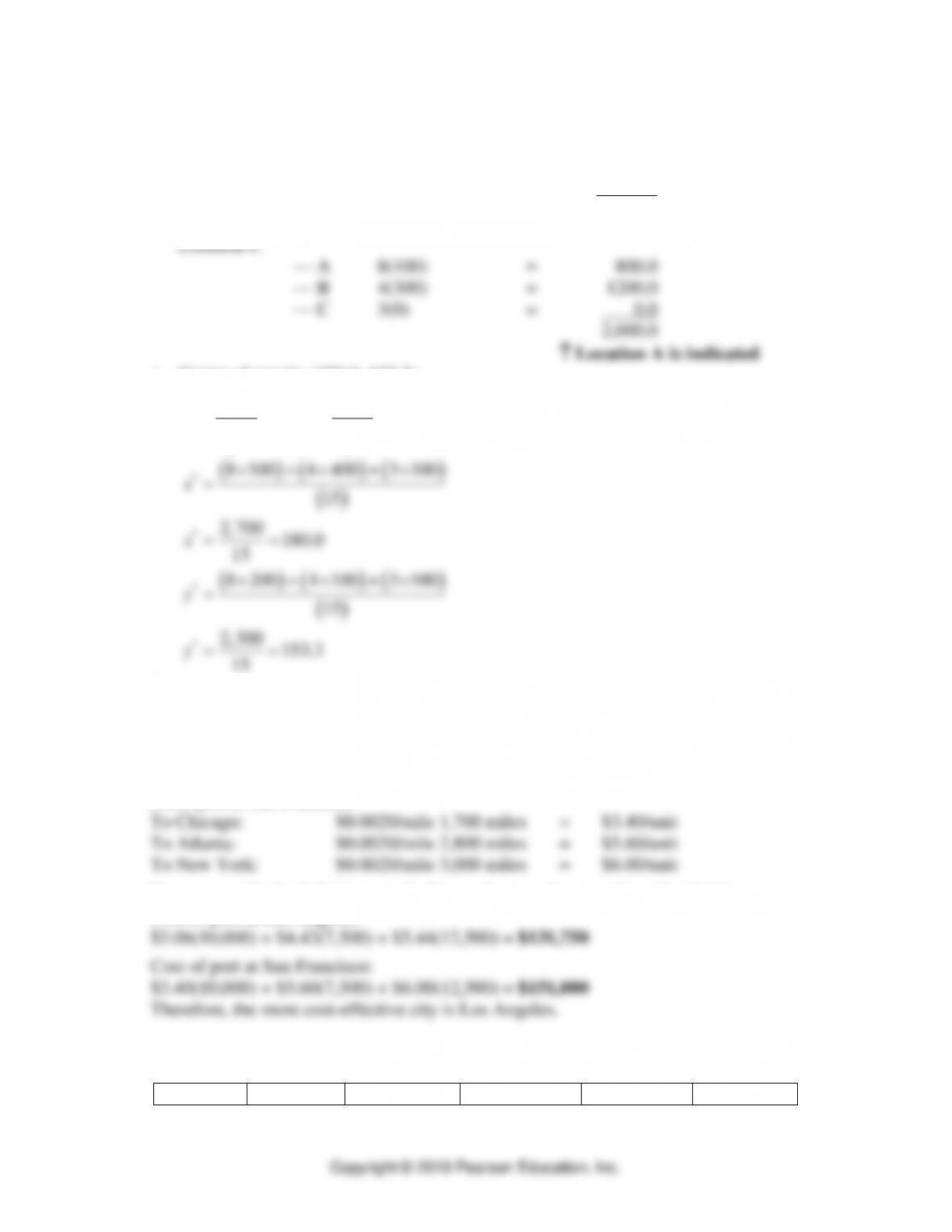
Supply Chain Logistic Networks ⚫ CHAPTER 13 ⚫
Location B
— A
8(400)
=
3,200.0
— B
4(0)
=
0.0
— C
3(300)
=
900.0
4,100.0
— A
8(100)
=
800.0
— B
4(300)
=
1200.0
— C
3(0)
=
0.0
2,000.0
c. Center of gravity (180.0, 153.3)
x
l x
l
i i
i
i
i
*=
and
y
l y
l
i i
i
i
i
*=
( ) ( ) ( )
( )
( ) ( ) ( )
( )
*
*
*
*
8 100 4 400 3 100
15
2,700 180.0
15
8 200 4 100 3 100
15
2,300 153.3
15
x
x
y
y
+ +
=
==
+ +
=
==
6. Personal computer manufacturer
From port at Los Angeles:
To Chicago: $0.0017/mile 1,800 miles = $3.06/unit
To Atlanta: $0.0017/mile 2,600 miles = $4.42/unit
To New York: $0.0017/mile 3,200 miles = $5.44/unit
From port at San Francisco:
Now we use the load-distance method to evaluate each port, where ld = i lidi
Cost of port at Los Angeles:
7. Oscar’s Bowling Inc.
a. Center of gravity
City
Population
x
y
Pop * x
Pop * y
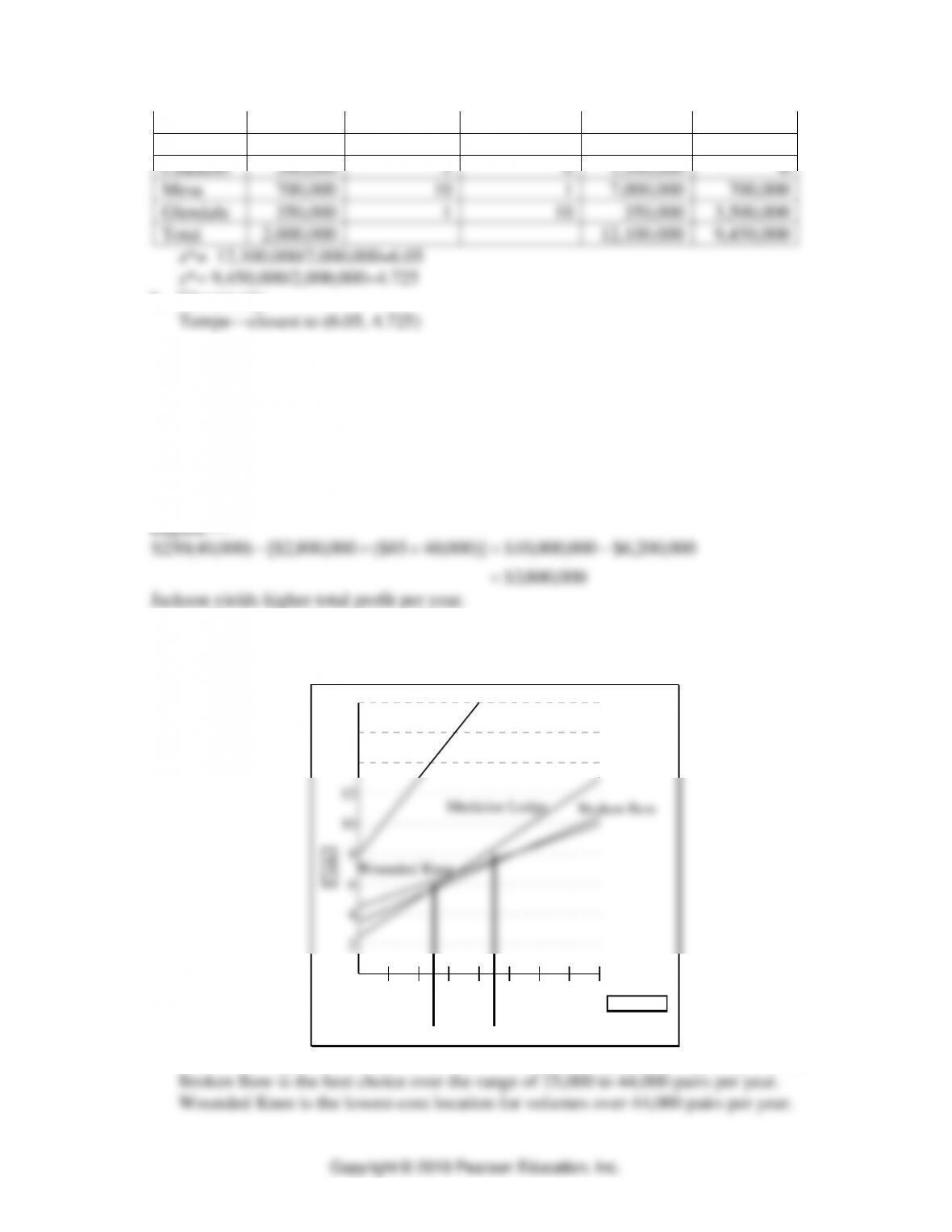
⚫ PART 3 ⚫ Managing Supply Chains
Tempe
250,000
5
5
1,250,000
1,250,000
Scottsdale
400,000
5
10
2,000,000
4,000,000
Chandler
300,000
5
0
1,500,000
0
Mesa
700,000
10
1
7,000,000
700,000
Glendale
350,000
1
10
350,000
3,500,000
Total
2,000,000
12,100,000
9,450,000
b. Closest city
Break-Even Analysis
8. Jackson or Dayton locations
Jackson —
$250(30,000) [$1,500,000 ($50 30,000)] $7,500,000 $3,000,000
$4,500,000
− + = −
=
9. Fall-Line, Inc.
a. Plot of total costs (in $ millions) versus volume (in thousands)
14
12
10
8
6
4
2
18
16
0
Aspen
Medicine Lodge Broken Bow
Wounded Knee
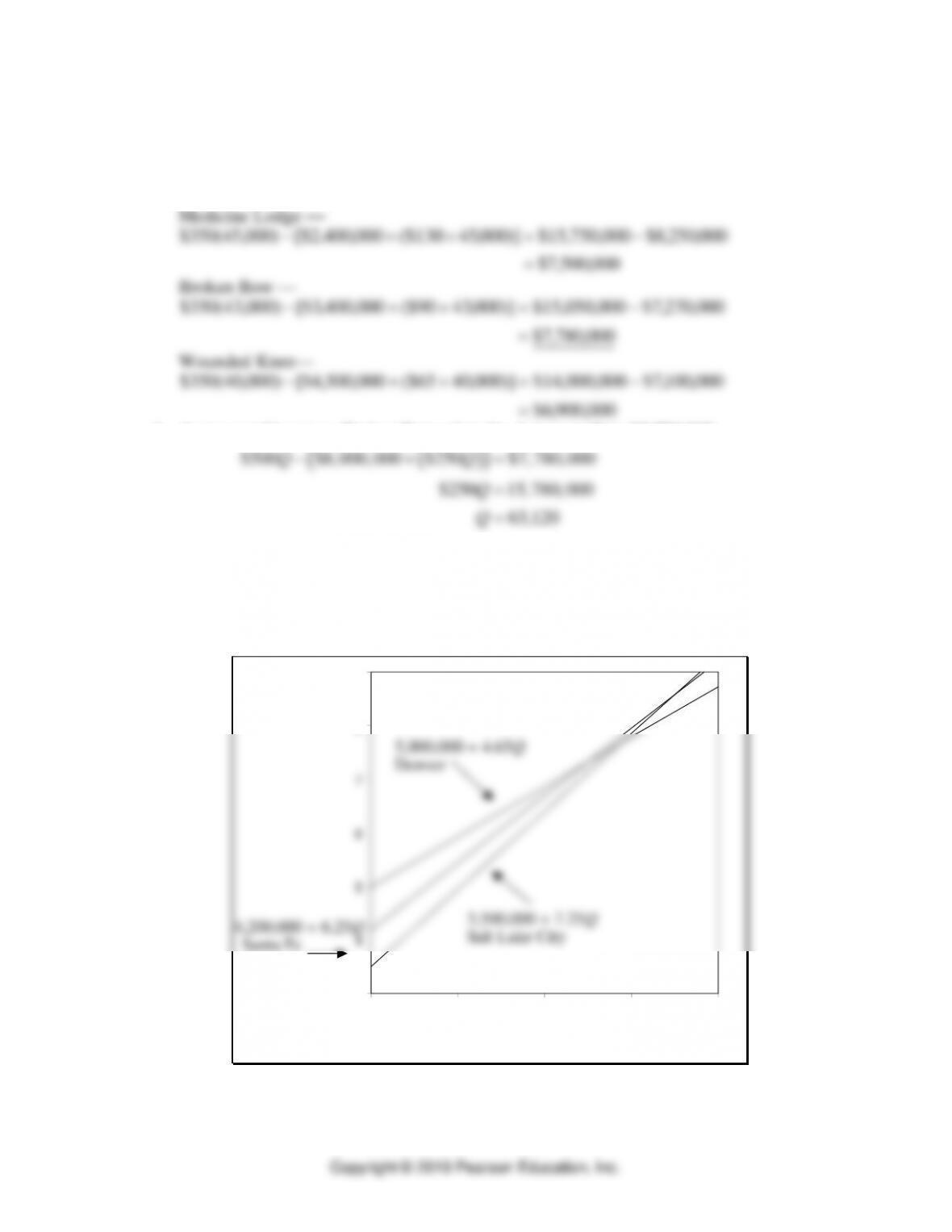
Supply Chain Logistic Networks ⚫ CHAPTER 13 ⚫
Aspen is not the low-cost location at any volume.
c. Aspen —
$500( , ) [$8, , ($250 , )] $30, , $23, ,
$7,
60 000 000 000 60 000 000 000 000 000
000 000
− + = −
=,
$6,
900 000
=,
d. Aspen would surpass Broken Bow when the Aspen profit is $7,780,000.
( )
( )
$500 $8, 000, 000 $250 $7,780,000
$250 15,780,000
63,120
QQ
Q
Q
− + =
=
=
Aspen would be the best location if sales would exceed 63,120 pairs per year. Holding
all other sales volumes constant.
10. Wiebe Trucking, Inc.
a. Plot of total costs (in $ millions) versus volume (in thousands)
3
4
5
6
7
8
9
0200 400 600 800
Volume
4,200,000 + 6.25
Santa Fe
5,000,000 + 4.65
Denver
3,500,000 + 7.25
Salt Lake City
576.9
QQ
Q
b. For up to 576,923 shipments per year, Salt Lake City is the best location. Beyond that,
⚫ PART 3 ⚫ Managing Supply Chains
11. Sam’s Bagels
Expected annual profits from “Downtown” location:
12. Dennison Manufacturing.
a.
Breakeven quantity between Phoenix and Buffalo =
(600,000-300,000)/(75-60)= 20,000 units
Seattle for more than 40,909 units
Transportation Method
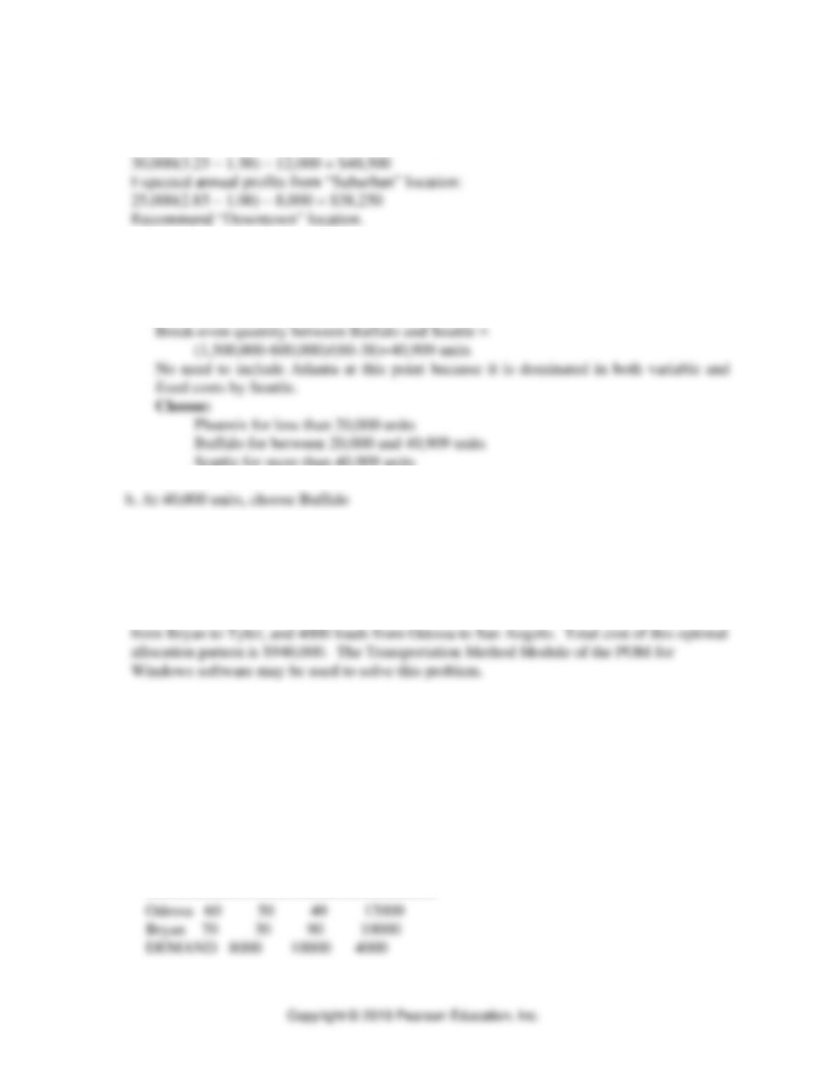
13. Prescott Industries
The cost minimizing solution is to ship 8000 loads from Odessa to Abilene, 10000 loads
Solution from POM for Windows
Module/submodel: Transportation Method (Location)
Problem title: Prescott Industries
Objective: Minimize
Data and Results ———-
Original Data
Abilene Tyler San Angelo Capacity
—————————————-————–
Supply Chain Logistic Networks ⚫ CHAPTER 13 ⚫
Shipments
Abilene Tyler San Angelo
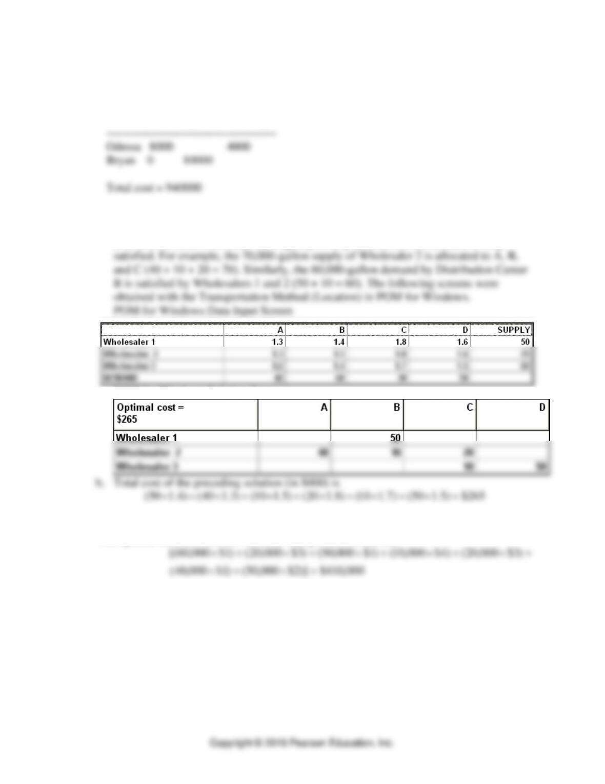
14. Winston Company
a. The sum of supply capacities equals the sum of demands, so no dummy wholesaler or
distribution center is needed. The capacity is fully utilized and the demand is fully
POM for Windows Solution Screen
15. The Acme Company
The optimal solution follows. The total transportation costs are:
000,410$)]2$000,50()1$000,40(
)3$000,20()4$000,10()1$000,50()3$000,20()1$000,60[(
=+
+++++
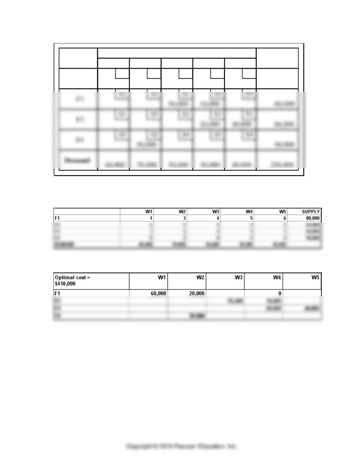
⚫ PART 3 ⚫ Managing Supply Chains
Factory Shipping Cost ($/case) to Warehouse
W1 Capacity
F1
Demand
$1
$2
60,000 250,000
80,000
60,000
$1
60,000
F2
F3
W2
$3
$2
70,000
$5
W3
$4
$1
60,000
50,000
$1
W4
$5
$4
20,000
30,000
$3
$5
50,000
F4 $2 $4 $5
W5
$6
$5
40,000
$1
$4
50,000 10,000
20,000 40,000
50,000
These results can be obtained with the Transportation Method (Location) module in POMS
for Windows:
Data Screen
Solution Screen
Supply Chain Logistic Networks ⚫ CHAPTER 13 ⚫
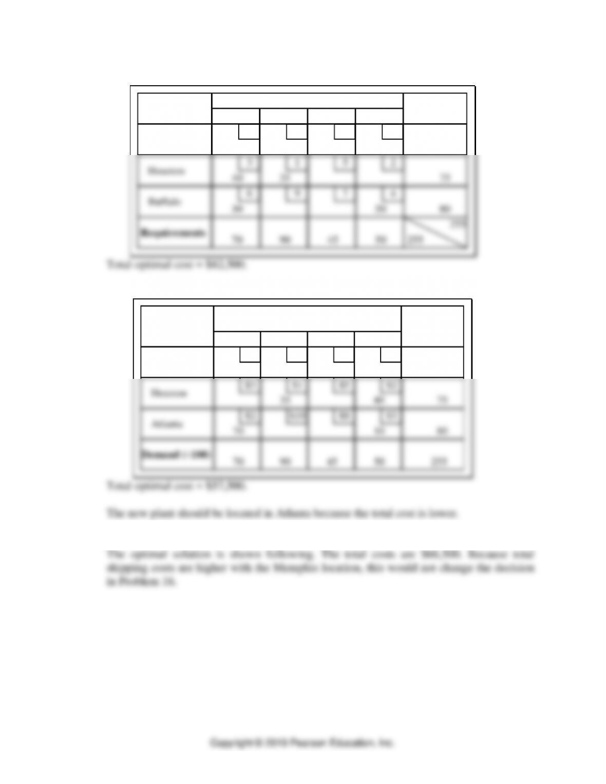
Buffalo location-optimal solution:
Plant Distribution Center
Miami Capacity
Chicago
Requirements
7
3
40
70 255
100
75
6
80
Houston
Buffalo
Denver
2
1
50
90
9
Lincoln
4
5
45
45
7
Jackson
5
2
50
4
255
35
30
55
Atlanta location-optimal solution:
Plant
Shipping cost to Distribution Centers
Miami
Capacity
Chicago
Demand ( 100)
$7
$3
70 255
100
75
$2
80
Houston
Atlanta
Denver
$2
$1
10
90
$10
Lincoln
$4
$5
45
45
$8
Jackson
$5
$2
50
$3
35
70
55
($/case) ( 100)
40
Total optimal cost = $57,500.
The new plant should be located in Atlanta because the total cost is lower.
17. Giant Farmer Company: Further Analysis—Memphis Plant
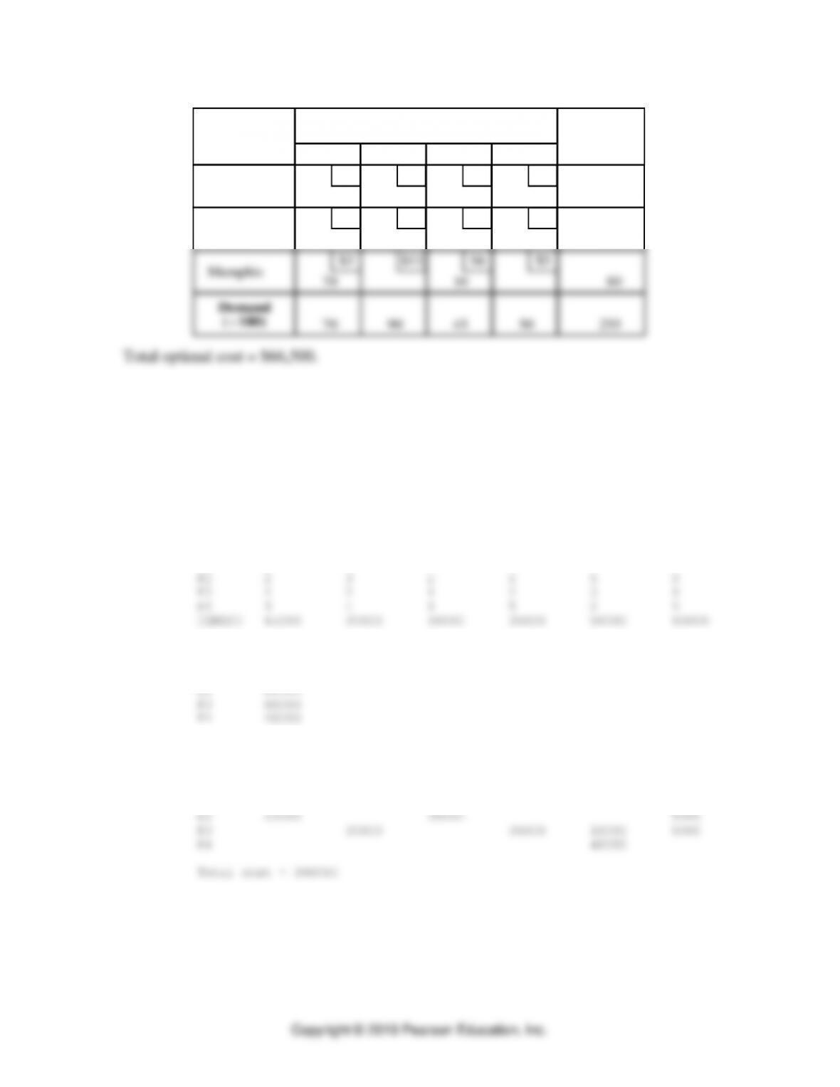
⚫ PART 3 ⚫ Managing Supply Chains
Supplier
Shipping cost to Distribution Centers
Miami
Capacity
Chicago $7
$3
70 255
100
75
$3
80
Houston
Memphis
Denver
$2
$1
10
90
$11
Lincoln
$4
$5
35
45
$6
Jackson
$5
$2
50
$5
25
70
65
($/case) ( 100)
50
Demand
( 100)
18. Thor International Company
Using the Transportation Method (Location) module in POMS for Windows, the optimal
solution is found to be:
Module/submodel: Transportation Method (Location)
Problem title: Thor International
Objective: Minimize
Original Data
W1 W2 W3 W4 W5 Dummy
————————————————————————-
F1 2 3 3 2 6 0
Capacity
———————
F1 50000
DEMAND
Shipments
W1 W2 W3 W4 W5 Dummy
————————————————————————-
F1 50000
A dummy warehouse with a demand of 60,000 units was added, because plant capacities
exceeded total demand by that amount. Note that Factory 1 ships its entire capacity to the