
Chapter
10 Operations Planning and Scheduling
TEACHING TIP
Open with Cooper Tire and Rubber Company. This example shows how employee hires, changes
to workforce schedules, temporary use of undertime by idling a plant, and facility scheduling can
be used to achieve strategic initiatives.
1. This chapter focuses on two major parts
a. Sales and operations planning
b. Scheduling
2. Requires managerial inputs from all of the firm’s functions
a. Marketing provides inputs demand and customer requirements.
b. Accounting provides cost data and the firm’s financial condition.
3. Each function is affected by the plan.
a. Plan calls for expanding or reducing the workforce has a direct impact on hiring and
training requirements for the human resources function.
b. As the plan is implemented, it creates revenue and cost streams that finance must deal
with as it manages the firm’s cash flow.
c. Each department and group in a firm has its own workforce.
• Managers of these departments must make choices on hiring, overtime, and
vacations.
4. Types of plans with operations planning and scheduling
a. Sales and operations plan (S&OP): A plan of future aggregate resource levels so that
supply is in balance with demand.
b. Aggregate plan: Another term for the sales and operations plan.
c. Production plan: A sales and operations plan for a manufacturing firm.
d. Staffing plan: A sales and operations plan for a service firm.
e. Resource plan: Determines requirements for materials and other resources on a more
detailed level than the S&OP.
f. Schedule: A detailed plan that allocates resources to accomplish specific tasks.
1. Levels in Operations Planning and Scheduling
1. Level 1: Sales and Operations Planning
a. Aggregation
• Product families
A group of customers, services, or products that have similar demand
requirements and common process, labor, and materials requirements.
Sometimes, product families relate to market groupings or to specific processes.
A firm can aggregate its services or products into a set of relatively broad
families, avoiding too much detail at this stage of the planning process.
• Workforce
• Time
Planning horizon typically one year.
Adjustments usually are made monthly or quarterly.
b. Information inputs
c. The relationship of operations plans and schedules to other plans
• A business plan is a projected statement of income, costs, and profits.
• An annual plan or financial plan is used by a nonprofit service organization.
2. Level 2: Resource Planning
The next planning level is resource planning to determine the firm’s workforce schedules
and other resource requirements.
a. Resource planning for manufacturing firms
• Master production schedule
• Materials requirements planning
b. Resource planning for services

• Daily or weekly capacity requirements for facilities or labor.
3. Level 3: Scheduling
a. The lowest planning level is scheduling, which puts together day–to-day schedules for
individual employees and customers.
b. Facility schedules, workforce schedules, and the sequence of jobs on bottleneck
machines.
2. S&OP Supply Options
There are six options that can be used singly or in combination to arrive at a plan.
• Anticipation Inventory: can be used to absorb uneven rates of demand or supply.
• Workforce Adjustment: management can adjust workforce levels by hiring or laying off
employees.
• Workforce Utilization: an alternative to a workforce adjustment is a change in workforce
utilization
o Overtime: employees work longer than the regular workday or workweek and
receive additional pay for the extra hours
o Undertime: employees do not have enough work for the regular-time workday or
workweek.
• Part-Time Workers: who are paid only for the hours and days worked
• Subcontractors: can be used to overcome short-term capacity shortages, such as during
peaks of the season or business cycle.
• Vacation Schedules: a manufacturer can shut down during an annual lull in sales, leaving
a skeleton crew to cover operations and perform maintenance.
3. S&OP Strategies
1. Two basic strategies are useful starting points in searching for the best plan.
a. Chase strategy
• Involves hiring and laying off employees to match the demand forecast over the
planning horizon.
• Requires no inventory investment, overtime, or undertime.
• The drawbacks are the expense of continually adjusting workforce levels, the
potential alienation of the workforce, and the possible loss of productivity and quality
because of constant changes in workforce.
b. Level strategy
• Involves keeping the workforce constant
• Utilization varies to match the demand forecast via overtime, undertime, and vacation
planning.
c. Mixed strategy

• Considers and implements a fuller range of reactive alternatives than either “pure”
strategy.
2. Constraints and costs
a. Constraints
• Physical limitations
• Managerial policies
b. Types of costs
• Regular-time costs
• Overtime costs
• Hiring and layoff costs
• Inventory holding costs
• Backorder and stockout costs
3. Sales and operations planning as a process
a. Involves planners and managers
b. Six basic step process typically done on a monthly basis (much like the steps discussed in
Chapter 13, “Forecasting.”
• Step 1: “roll forward” the plan for the new planning horizon and update files with
actual sales, production, inventory, costs, and constraints
• Step 2: forecast and demand planning
• Step 3: update sales and operations planning spreadsheet for each family
• Step 4: consensus meeting
• Step 5: executive sales and operations planning meeting
• Step 6: update the spreadsheets to reflect the authorized plan and communicate the
plans to the important stakeholders for implementation
4. Spreadsheets for Sales and Operations Planning
1. Spreadsheets for a manufacturer (demonstrate with the Sales and Operations Planning
with Spreadsheets Solver in OM Explorer)
• Input values: the forecasted demand requirements and the supply option choices
period by period
express the forecasted demand and supply options as employee-period
equivalents.
• Derived values:
utilized time: that portion of the workforce’s regular time that is paid for and
productively used
inventory: can be calculated by subtracting the forecast from the utilized time,
adding last periods ending inventory, and adding subcontracting time and
backorders.
hires and layoffs: can be derived from the workforce levels
undertime and overtime: are shown as input values (rather than derived values) in
the spreadsheet
• Calculated values: shows the plan’s cost consequences.
2. Spreadsheets for a service provider
a. Service providers can use the same spreadsheets, except anticipation inventory is not an
option.
3. Data for Applications 10.1-10.3 for comparing strategies
The Barberton Municipal Division of Road Maintenance is charged with road repair in the
city of Barberton and surrounding area. Cindy Kramer, road maintenance director, must
submit a staffing plan for the next year based on a set schedule for repairs and on the city
budget. Kramer estimates that the labor hours required for the next four quarters are 6,000,
12,000, 19,000, and 9,000, respectively. Each of the 11 workers on the workforce can
contribute 520 hours per quarter. Overtime is limited to 20 percent of the regular-time
capacity in any quarter. Subcontracting is not permitted.
Payroll costs are $6,240 in wages per worker for regular time worked up to 520 hours,
with an overtime pay rate of $18 for each overtime hour. Although unused overtime capacity
has no cost, unused regular time is paid at $12 per hour. The cost of hiring a worker is
$3,000, and the cost of laying off a worker is $2,000.
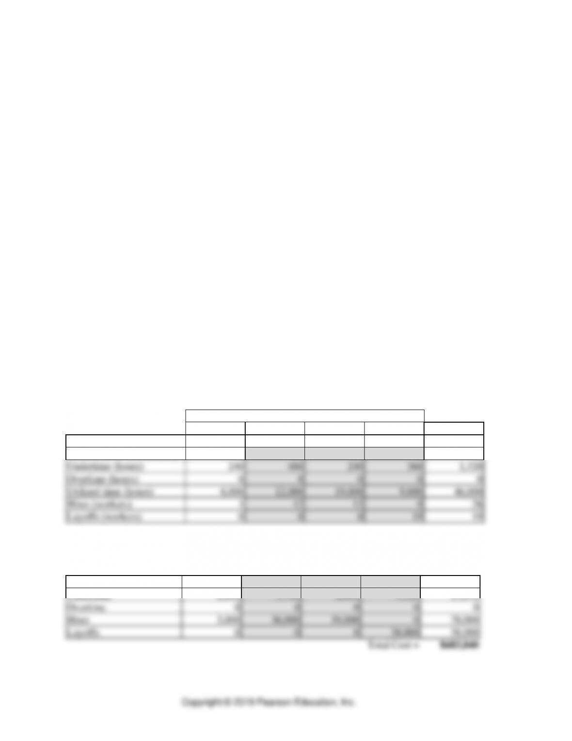
a. Application 10.1: Chase Strategy
Use a chase strategy for the Barberton Municipal Division that varies the workforce level
without using overtime. Undertime should be minimized, except for the minimal amount
mandated because the quarterly requirements are not integer multiples of 520 hours.
(Students complete highlighted sections)
Quarter
1
2
3
4
Total
Forecasted demand (hrs)
6,000
12,000
19,000
9,000
46,000
Workforce level (workers)
12
24
37
18
91
Undertime (hours)
240
480
240
360
1,320
Overtime (hours)
0
0
0
0
0
Utilized time (hours)
6,000
12,000
19,000
9,000
46,000
Hires (workers)
1
12
13
0
26
Layoffs (workers)
0
0
0
19
19
What is the total cost of this plan?
Costs
Utilized time
$72,000
$144,000
$228,000
$108,000
$552,000
Undertime
2,880
5,760
2,880
4,320
15,840
Overtime
0
0
0
0
0
Hires
3,000
36,000
39,000
0
78,000
Layoffs
0
0
0
38,000
38,000
Total Cost =
$683,840
b. Tutor 10.1 in MyLab Operations Management provides a new example for planning
using the chase strategy with hiring and layoffs.
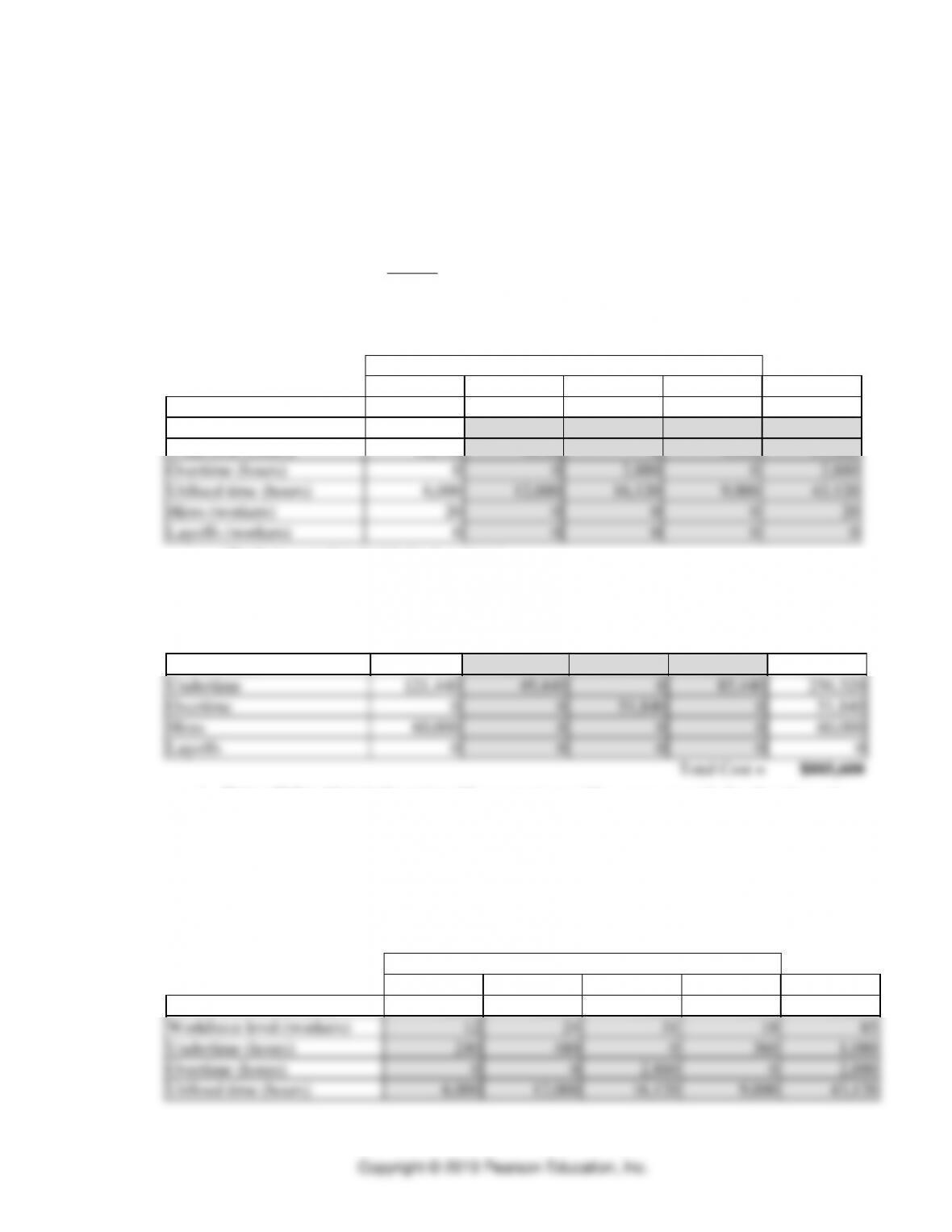
c. Application 10.2: Level Strategy
Find a level plan for the Barberton Municipal Division that allows no delay in road repair
and minimizes undertime. Overtime can be used to its limits in any quarter. Given that
the demand peaks in quarter 3, we get:
1.20w =
520
000,19
= 36.54 employee-period equivalents
w = 30.45 or 31 employees
Quarter
1
2
3
4
Total
Forecasted demand (hrs)
6,000
12,000
19,000
9,000
46,000
Workforce level (workers)
31
31
31
31
124
Undertime (hours)
10,120
4,120
0
7,120
21,360
Overtime (hours)
0
0
2,880
0
2,880
Utilized time (hours)
6,000
12,000
16,120
9,000
43,120
Hires (workers)
20
0
0
0
20
Layoffs (workers)
0
0
0
0
0
(Students complete highlighted sections)
What is the cost of this level workforce plan?
Costs
Utilized time
$72,000
$144,000
$193,440
$108,000
$517,440
Undertime
121,440
49,440
0
85,440
256,320
Overtime
0
0
51,840
0
51,840
Hires
60,000
0
0
0
60,000
Layoffs
0
0
0
0
0
Total Cost =
$885,600
d. Tutor 10.2 in MyLab Operations Management provides a new example for planning and
using the level strategy with overtime and undertime.
e. Application 10.3: Mixed Strategy to consider and implement a fuller range of reactive
alternatives than any one “pure” strategy.
Now propose a plan of your own for the Barberton Municipal Division. Use the chase
strategy as a base, but find a way to decrease the cost of hiring and layoffs by selectively
using some overtime. (Students complete highlighted sections)
Quarter
1
2
3
4
Total
Forecasted demand (hrs)
6,000
12,000
19,000
9,000
46,000
Workforce level (workers)
12
24
31
18
85
Undertime (hours)
240
480
0
360
1,080
Overtime (hours)
0
0
2,880
0
2,880
Utilized time (hours)
6,000
12,000
16,120
9,000
43,120

Hires (workers)
1
12
7
0
20
Layoffs (workers)
0
0
0
13
13
Several solutions are possible. The key idea in creating this one is hiring only 7
employees in quarter 3, while using overtime to its maximum limit and eliminating
undertime for that quarter. Hiring fewer in quarter 3 allows the number of layoffs in
quarter 4 to drop to only 13, down from 19.
What is the cost of your mixed strategy plan?
Costs
Utilized time
$72,000
$144,000
$193,440
$108,000
$517,440
Undertime
2,880
5,760
0
4,320
12,960
Overtime
0
0
51,840
0
51,840
Hires
3,000
36,000
21,000
0
60,000
Layoffs
0
0
0
26,000
26,000
Total Cost =
$668,240
f. Tutor 10.4 in MyLab Operations Management provides another example for practicing
sales and operations planning using a variety of strategies (note: this is Solved Problem
1).
g. Active Model 10.1 in MyLab Operations Management shows the impact of changing the
workforce level, the cost structure, and overtime capacity.
5. Scheduling
TEACHING TIP
Scheduling is the last step. It takes the operation and scheduling process from planning to
execution, and where the “rubber meets the road.”
1. Job and Facility Scheduling
a. Gantt charts
• The progress chart: graphically displays the current status of each job or activity
relative to its scheduled completion date
• The workstation chart: can be used to schedule the capacity of facilities.
2. Workforce Scheduling
a. Translate the staffing plan into specific schedules of work for each employee
b. Constraints
• Technical constraints imposed on the workforce schedule are the resources provided
by the staffing plan and requirements placed on the operating system.
• Legal and behavioral considerations
• Psychological needs of workers

• Rotating schedule
Over a period of time, each person has the same opportunity to have weekends
and holidays off and to work days, as well as evenings and nights
• Fixed schedule
Calls for each employee to work the same days and hours each week.
c. Developing a workforce schedule
• Steps (example of workforce schedule for a company operating seven days a week
and providing each employee two consecutive days off)
Step 1: find all the pairs of consecutive days
Step 2: if a tie occurs, choose one of the tied pairs, consistent with the provisions
written into the labor agreement, if any
Step 3: assign the employees for the selected pair of days off
Step 4: repeat steps 1-3 until all of the requirements have been satisfied
• Quickly review Example 10.2: Developing a Workforce Schedule
• Tutor 10.3 in MyLab Operations Management provides a new example to practice
workforce scheduling.
TEACHING TIP
Use Managerial Practice 10.1 “Scheduling Major League Baseball Umpires” to illustrate how
workforce scheduling translates the staffing plan and time-based staffing requirements into work
schedules for each employee based upon, respectively, the number of MLB umpire crews, the
schedule of MLB games, and the umpire crew assignments to series.
3. Sequencing Jobs at a Workstation
a. Priority sequencing rules
• First-come, first-served (FCFS)
Example 10.3 Using the FCFS Rule
• Earliest due date (EDD)
b. Performance measures
• Flow time: the sum of the waiting time for servers or machines; the process time,
including setups; the time spent moving between operations; and delays resulting
from machine breakdowns, unavailability of facilitating goods or components, and
the like.
• Past due (also referred to as tardiness)
c. Application 10.4 (note: this is Solved Problem 3)
A consulting company has five jobs in its backlog. A schedule was created using the
FCFS rule and the average days past due was 3.4 days and the average flow time was
60.2 days. Create a new schedule using the EDD rule, calculating the average days past
due and flow time. In this case, does EDD outperform the FCFS rule?
Customer
Time Since Order
Processing
Due Date

Arrived (days ago)
Time (days)
(days from now)
A
15
25
29
B
12
16
27
C
5
14
68
D
10
10
48
E
0
12
80
Solution
Customer
Sequence
Start
Time
(days)
Processing
Time
(days)
Finish
Time
(days)
Due
Date
Days
Past
Due
Days
Ago
Since
Order
Arrived
Flow
Time
(days)
B
0
+
16
=
16
27
0
12
28
A
16
+
25
=
41
29
12
15
56
D
41
+
10
=
51
48
3
10
61
C
51
+
14
=
65
68
0
5
70
E
65
+
12
=
77
80
0
0
77
(Students will complete the shaded area. The bolded due dates represents the EDD
sequence. Likewise, the bolded flow time is calculated. Both are needed for the
performance measures.)
The days past due and average flow time performance for the EDD schedule are:
003120++++
5
By both measures, EDD outperforms the FCFS (3.0 versus 3.4 past due and 58.4 versus
60.2 flow time). However, the solution found in part (b) of example 14.3 still has the
best average flow time of only 47.8 days.
4. Software support
a. Computerized scheduling systems are available to cope with the complexity of workforce
scheduling which comes from the need to evaluate the numerous possible alternatives
b. Software is also available for sequencing jobs at workstations
• Advance planning and scheduling (APS) systems: seek to optimize resources across
the supply chain and align daily operations with strategic goals.