CHAPTER 15
Sourcing Decisions in a Supply Chain
1. EXCEL Worksheet 15-1 illustrates these computations:
With no buyback: See worksheet 15-1 a&b
Expected profits for Barnes & Noble’s = (p − s)
NORMDIST((O −
)/
, 0, 1, 1)
Expected understock =
Given that:
Copyright © 2019 Pearson Education, Inc.
We reevaluate the profits for Barnes & Noble’s (with s = b = 8) and the publisher (with b = 5). In
the presence of buybacks for $5, we obtain the following order size, expected overstock, and
expected understock:
Expected profit for Barnes & Noble’s = $214,578 (Cell B31)
Expected profit for publisher = $236,506 (Cell B32)
Total supply chain profit = $451,084 (Cell B33)
Observe that buyback leaves both Barnes and Noble and the publisher better off. It makes sense
for the publisher to buy back at $5.
2. EXCEL Worksheet 15-2 illustrates these computations:
With no buyback: See worksheet 15-2 a&b
Given that:
Copyright © 2019 Pearson Education, Inc.
= 3,248 (Cell B29)
Expected understock =
Given that:
Studio’s sale price (c) = $10
3. EXCEL Worksheet 15-3 illustrates these computations:
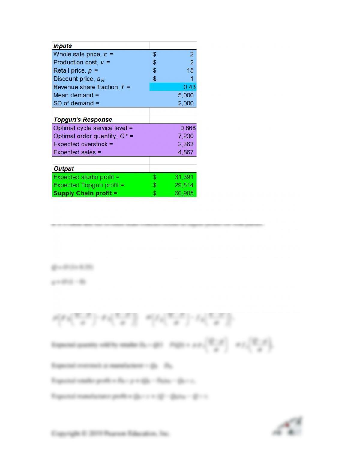
Topgun’s response: See worksheet 15-3 a,b,c,d
CSL =
)115)(35.01(
)315)(35.01(
)1(
)1(
−−
−−
=
−−
−−
=
+sCCC
Rou
u
pf
cpf
= 0.771 (Cell B22)
4. EXCEL Worksheet 15-4 illustrates these computations:
Expected quantity purchased by retailer, QR = qF(q) + Q(1 − F(Q)) +
−
−
−
q
F
Q
FSS
−
−
−
−
q
f
Q
fSS
,
Expected quantity sold by retailer DR = Q(1 − F(Q)) +
−
Q
FS
−
−
Q
fS
,
Expected overstock at manufacturer = QR − DR,
Expected retailer profit = DR p + (QR − DR)sR − QR c,
Expected manufacturer profit = QR c + (Q − QR)sM − Q v.
Copyright © 2019 Pearson Education, Inc.
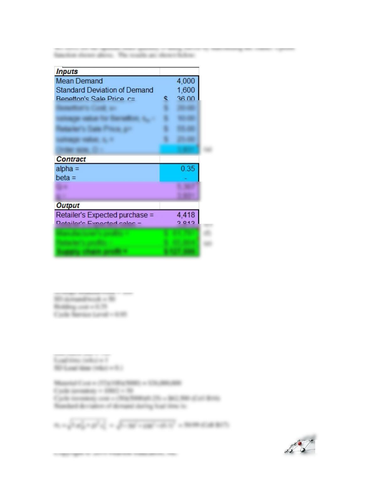
We solve for the optimal order quantity O using Solver by maximizing the retailer’s profit
function shown above. The results are shown below:
5. EXCEL Worksheet 15-5 illustrates these computations:
Supplier 1: Reliable (Cells A8:B21)
Cost/unit = $5,000
(a)
(b)
(c)
(f)
(e)
Supplier 2: Value (Cells D8:E21)
6. EXCEL Worksheet 15-6 illustrates these computations:
We reevaluate the total costs associated with supplier 2 based on the three options provided in the
problem; the costs are shown below:
Option
Spreadsheet Settings
Total Cost
LT = 4
Cell E9 = 1000, E10 = 4, E11 = 4
$26,373,828.55
min batch = 800
Cell E9 = 800, E10 = 5, E11 = 4
$26,259,790.75
SD of LT = 3
Cell E9 = 1000, E10 = 5, E11 = 3
$26,191,932.07
All three
Cell E9 = 800, E10 = 4, E11 = 3
$26,064,178.01
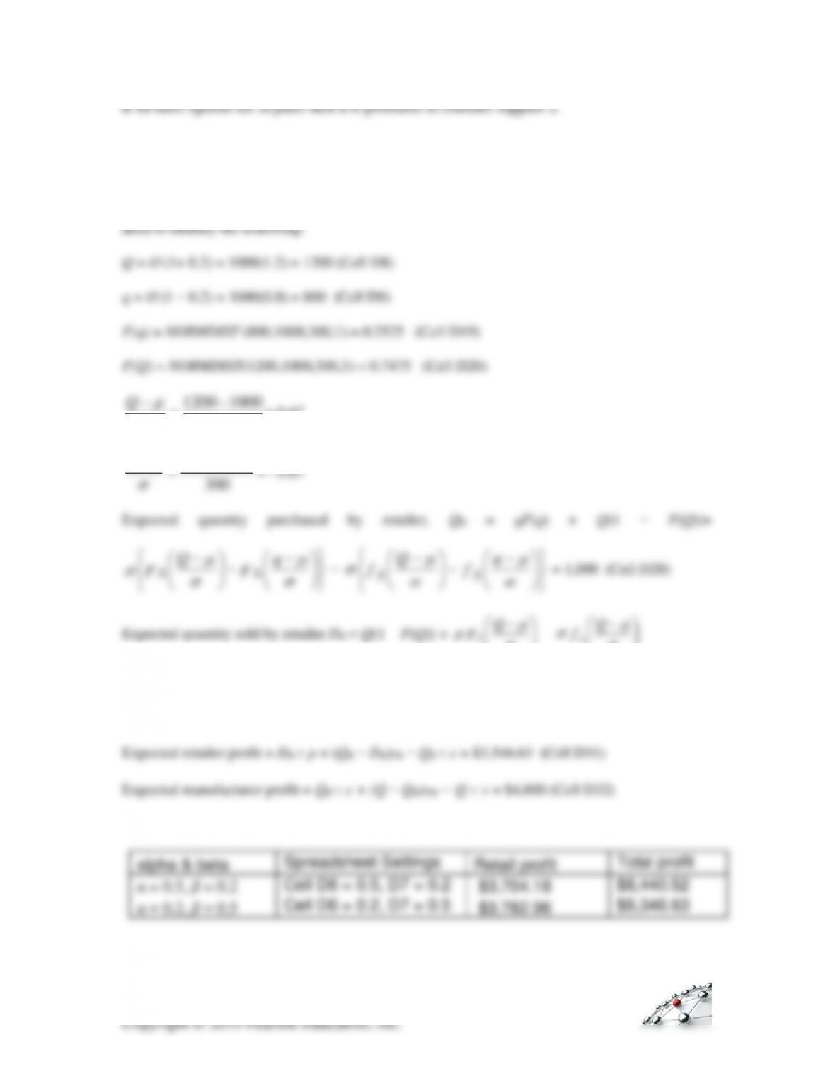
If all three options are in place then it is profitable to consider supplier 2.
7. EXCEL Worksheet 15-7 illustrates these computations:
The setup for this problem is same as problem 4 except that O is given in the problem and we
300
10001200−
=
−
Q
= 0.67
1000800−
−
q
8. EXCEL Worksheet 15-8 illustrates these computations:
If both the retailer and wholesaler are vertically integrated, profits (see Cell D34) can be calculated
8,346.63 (which is the same as when β = 0.2).
Observe that the quantity Q produced by the retailer only depends upon α and the expected quantity
sold by the retailer is not affected by q = O (1 − β). It is only affected by Q = O (1+ α). Thus, both