Chapter 13
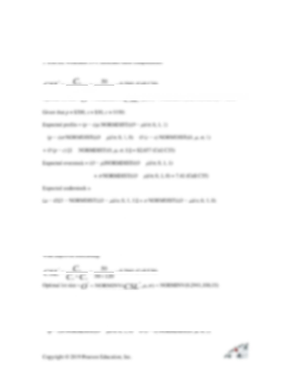
Exercise Solutions
=
+
=
+
=12050
50
*
CCC
CSL ou
u
0.2941 (Cell C30)
Optimal lot size =
**
NORMINV( , , )
O CSL
=
= NORMINV(0.2941,100,40) = 78.34
= 29.07 (Cell C36)
2. EXCEL worksheet 13-2 illustrates these computations:
=
+
=
+
=12050
50
*
CCC
CSL ou
u
0.2941 (Cell E30)
NORMINV( , , )
=
**
O CSL
= 91.88 (Cell E31)
Given that p = $200, s = $30, c = $150:
Expected profits = (p − s)
NORMDIST((O −
)/
, 0, 1, 1)
3. EXCEL worksheet 13-3 illustrates these computations:
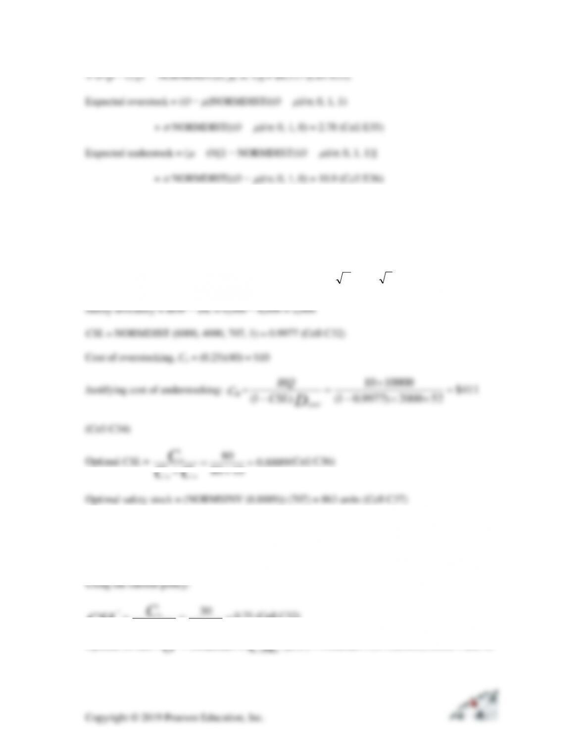
Mean demand during lead time =DL= (2000)(2) = 4,000 (Cell C26)
Standard deviation of demand during lead time = L =
L
D
= 500
2
= 707 (Cell C27)
4. EXCEL worksheet 13-4 illustrates these computations:
=
+
=
+
=1030
30
*
CCC
CSL ou
u
0.75 (Cell C32)
Optimal lot size =
**
NORMINV( , , )
O CSL
=
= NORMINV(0.75,20000,10000) = 26,745
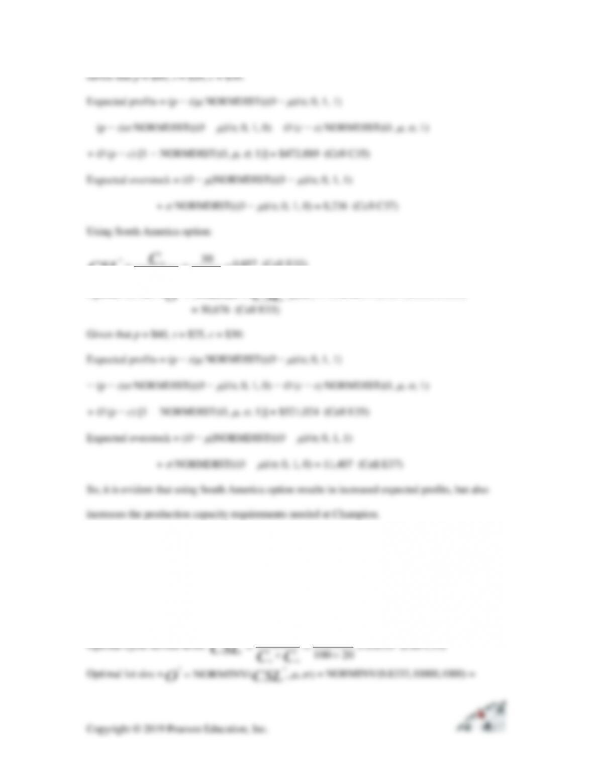
=
+
=
+
=530
30
*
CCC
CSL ou
u
0.857 (Cell E32)
Optimal lot size =
**
NORMINV( , , )
O CSL
=
= NORMINV(0.857,20000,10000)
5. EXCEL worksheet 13-5 illustrates these computations:
Current sourcing (one line):
Reguplo:
**
NORMINV( , , )
O CSL
=
100
*
u
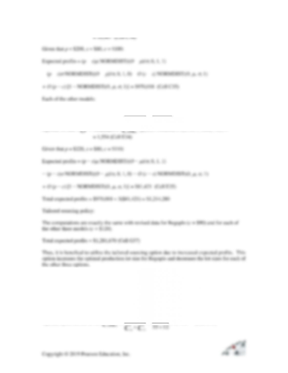
Optimal cycle service level,
=
+
=
+
=30110
110
*
CCC
CSL ou
u
0.7857 (Cell E33)
Optimal lot size =
),,(NORMINV **
CSLO =
= NORMINV(0.7857, 1000, 700) =
6. EXCEL worksheet 13-6 illustrates these computations:
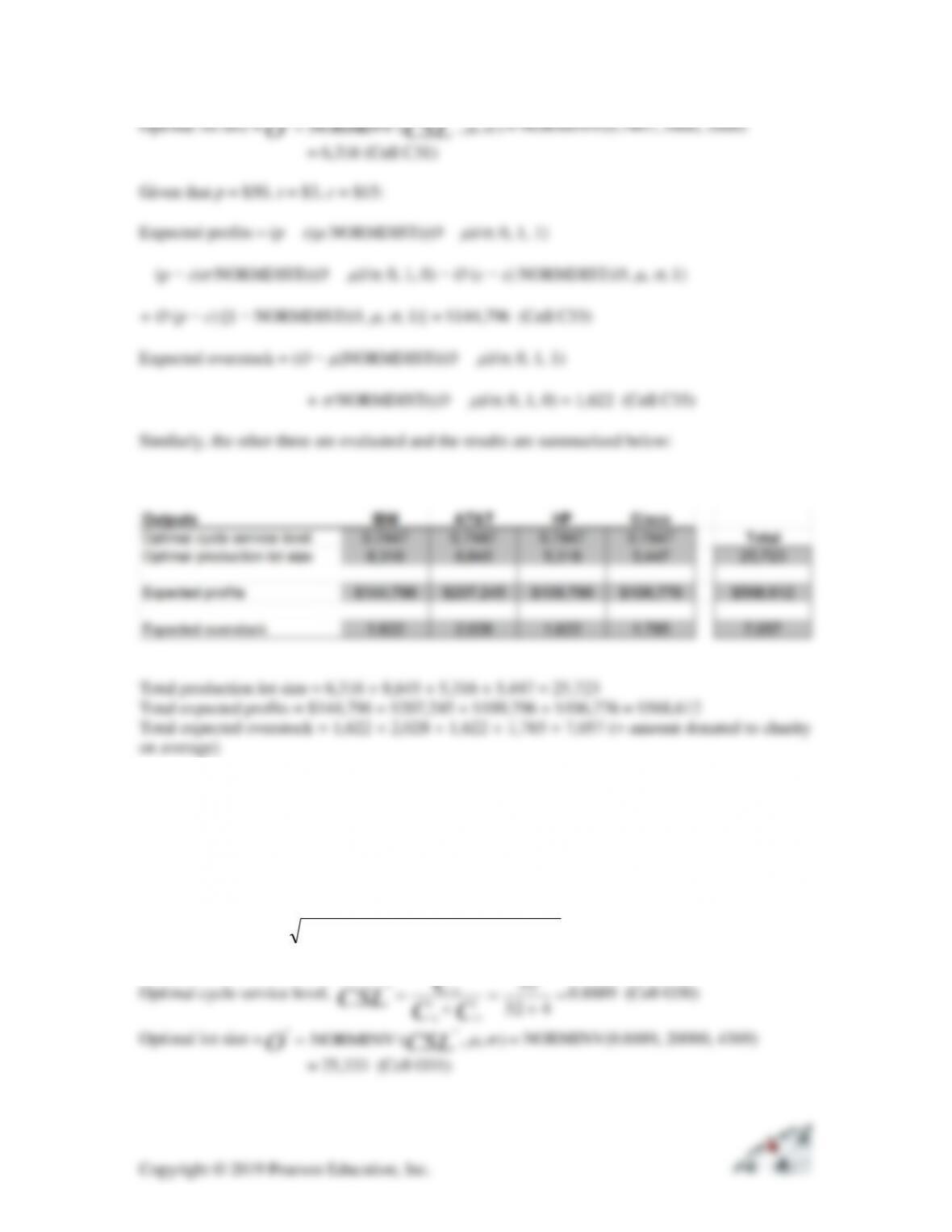
IBM:
Optimal cycle service level,
=
+
=
+
=1235
35
*
CCC
CSL ou
u
0.7447 (Cell C30)
7. EXCEL worksheet 13-7 illustrates these computations:
With aggregation:
Anticipated demand = 5,000 + 7,000 + 4,000 + 4,000 = 20,000 (Cell O17)
Standard deviation =
369,4200,2000,2500,2000,2 2222 =+++
(Cell O18)
32
*
u
8. EXCEL worksheet 13-8 illustrates these computations:
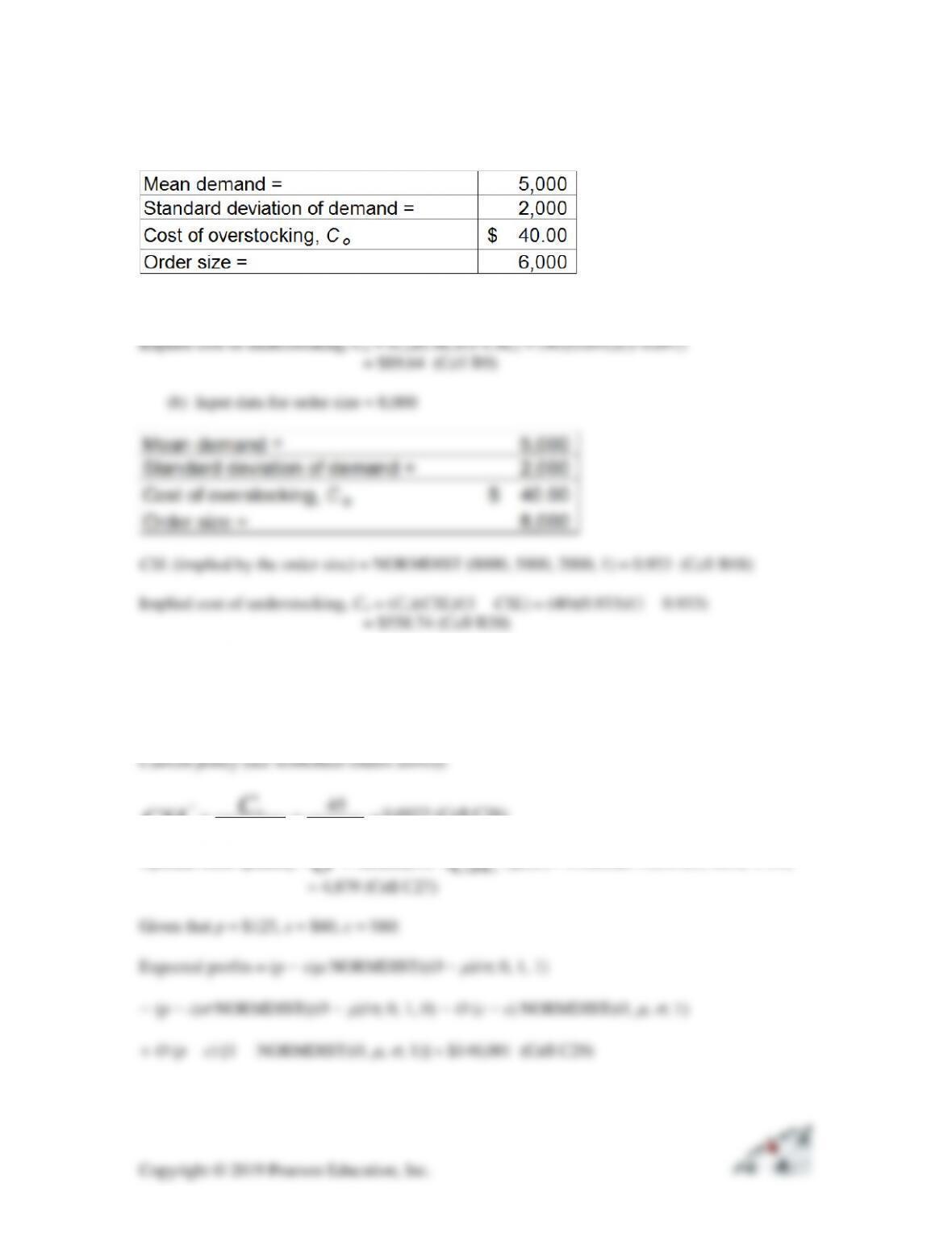
(a) Input data for order size = 6,000
CSL (implied by the order size) = NORMDIST (6000, 5000, 2000, 1) = 0.691 (Cell B7)
10. EXCEL worksheet 13–10 illustrates these computations:
=
+
=
+
=2045
45
*
CCC
CSL ou
u
0.6923 (Cell C26)
Optimal order quantity =
),,( **
CSLO NORMINV=
= NORMINV(0.6923, 4000, 1750)
=
+
=
+
=545
45
*
CCC
CSL ou
u
0.90 (Cell C26)
11. EXCEL worksheet 13–11 illustrates these computations:
(a) See worksheet 13.11a:
Mean demand during lead time = DL = (40)(1) = 40 (Cell C24)
Standard deviation of demand during lead time = L =
L
D
= 5
1
= 5 (Cell C25)
Safety inventory = ROP − DL = 45 − 40 = 5
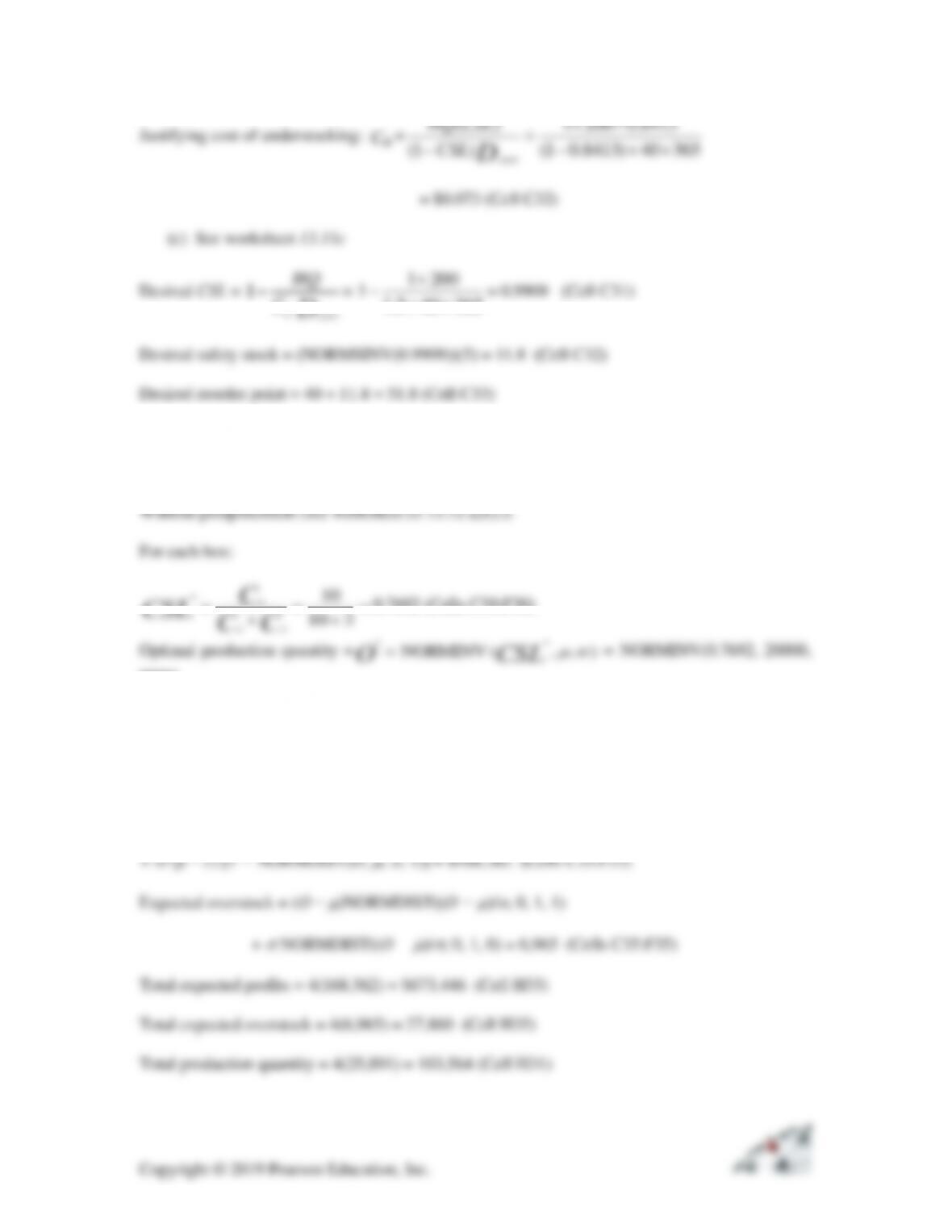
( ) 1 200 0.8413
HQ CSL
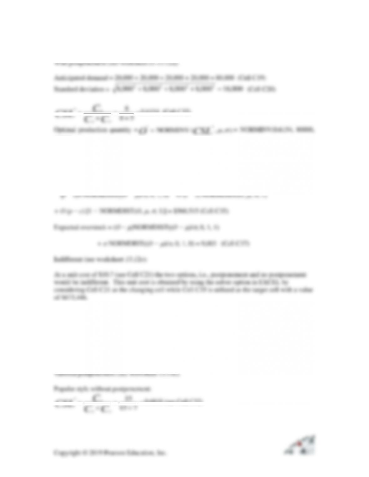
=
+
=
+
=58
8
*
CCC
CSL ou
u
0.6154 (Cell C32)
CSLO =
16000) = 84,694 (Cell C33)
Given that p = $20, s = $7, c = $12:
Expected profits = (p − s)
NORMDIST((O −
)/
, 0, 1, 1)
13. EXCEL worksheet 13–13 illustrates these computations:
The without postponement (see worksheet 13.13a,b,c) and with postponement (see worksheet
13.13d) calculations are similar to problem 12, but what is new in this problem is the tailored
postponement, which is discussed below:
=
+
=
+
=715
15
*
CCC
CSL ou
u
0.6818 (see Cell C32)
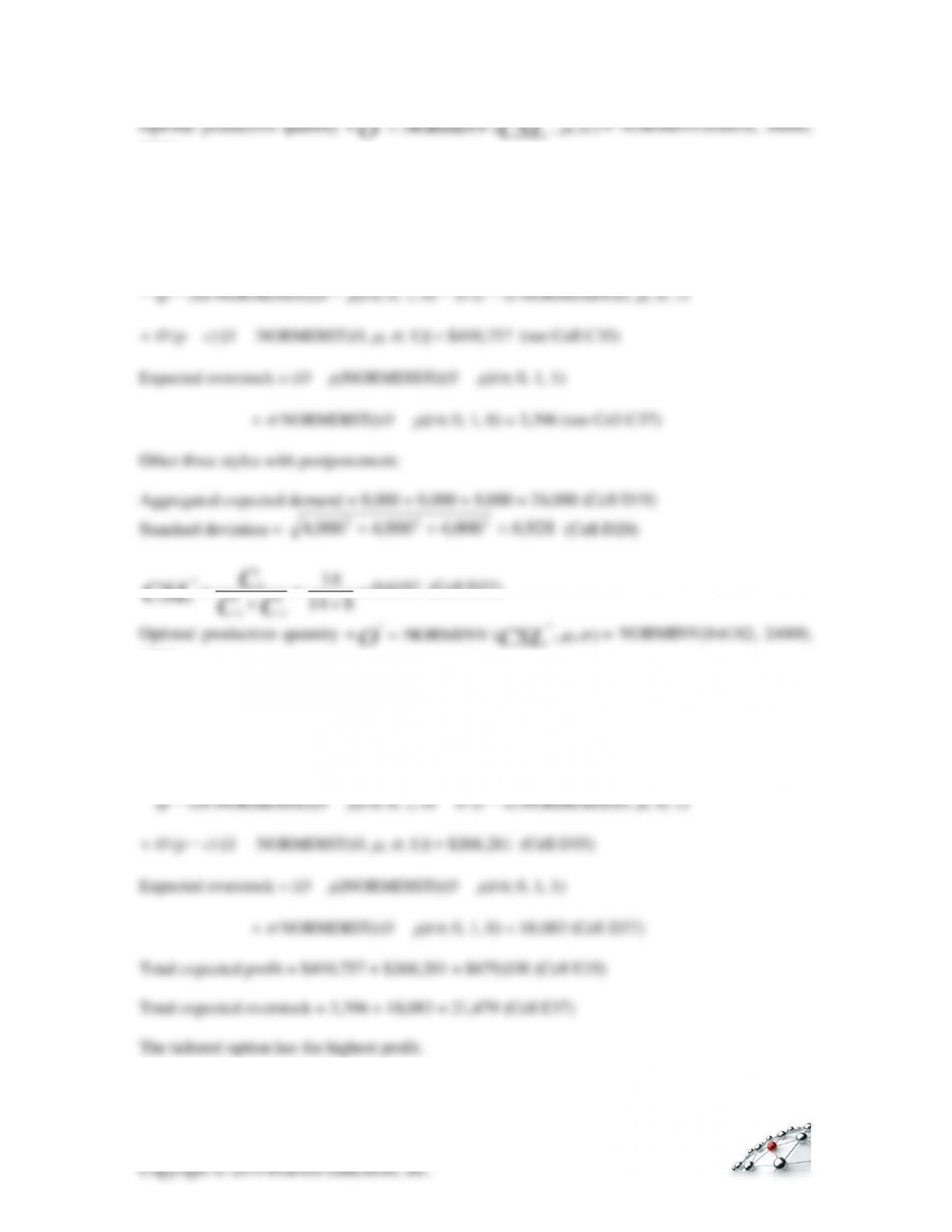
CSLO =
5000) = 32,364 (see Cell C33)
Given that p = $35, s = $13, c = $20:
Expected profits = (p − s)
NORMDIST((O −
)/
, 0, 1, 1)
=
+
=
+
=814
14
*
CCC
CSL ou
u
0.6182 (Cell D32)
CSLO =
6928) = 26,083 (Cell D33)
Given that p = $35, s = $13, c = $21.4:
Expected profits = (p − s)
NORMDIST((O −
)/
, 0, 1, 1)
14. EXCEL worksheet 13–14 illustrates these computations:
=
+
=
+
=3065
65
*
CCC
CSL ou
u
0.6842 (Cell B28)
Optimal order quantity =
),,(NORMINV **
CSLO =
= NORMINV(0.6842, 20000, 8000)
15. EXCEL worksheet 13–15 illustrates these computations:
=
+
=
+
=37
7
*
CCC
CSL ou
u
0.7 (Cell B28)
Optimal order quantity =
),,(NORMINV **
CSLO =
= NORMINV(0.7, 70000, 25000)
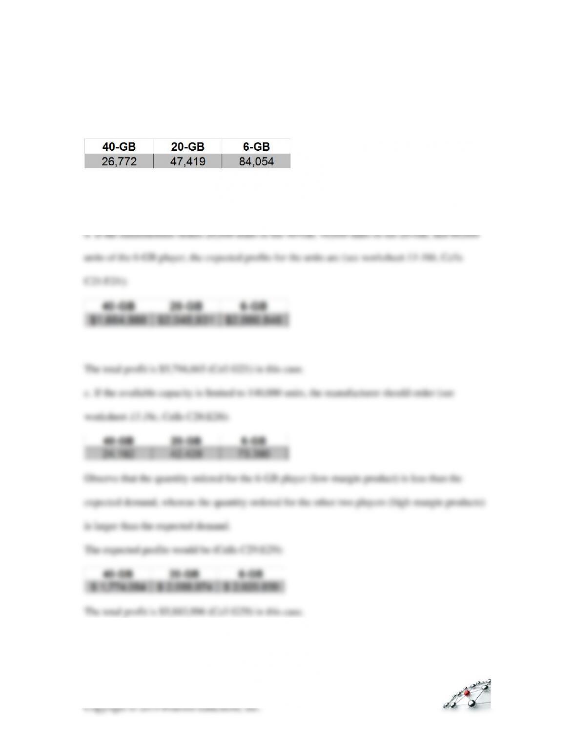
16. EXCEL worksheet 13–16 illustrates these computations:
a. Without capacity constraints, the manufacturer should order the following quantity of each
player (see worksheet 13–16a, Cells C19:E19):
The total profit is $6,001,408 (Cell G21) in this case.
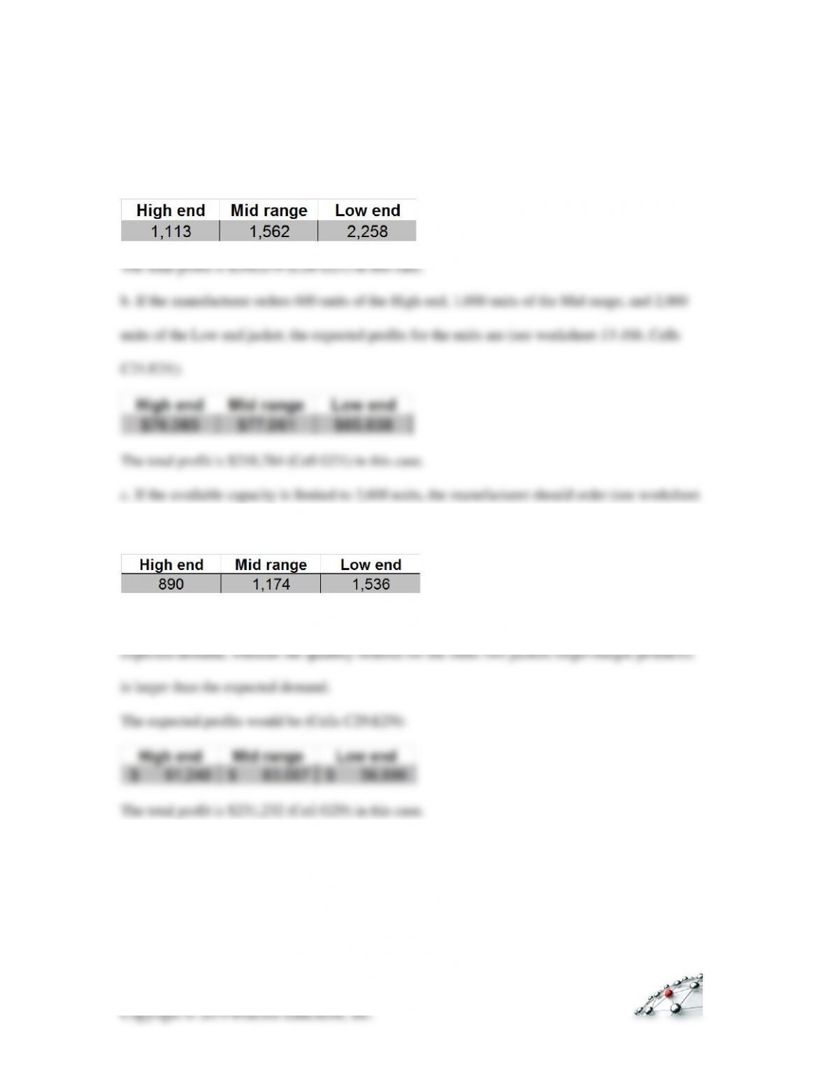
17. EXCEL worksheet 13-17 illustrates these computations:
a. Without capacity constraints, the manufacturer should order the following quantity of each
jacket (see worksheet 13-17a, Cells C19:E19):
13.16c, Cells C26:E26):
Observe that the quantity ordered for the Low end jacket (low-margin product) is less than the