1
Chapter 16: Pricing and Revenue Management in a Supply Chain
Exercise Solutions
1. Worksheet 16-1 presents this solution.
The amount of production capacity to reserve is:
2. Worksheet 16-2 presents this solution:
Just as in the case of the previous problem:
3. Worksheet 16-3 presents this solution:
(a) See worksheet 16.3a
s* =
CC
C
sw
w
+
=
33
3
+
= 0.5 (Equation 16.6)
Copyright © 2019 Pearson Education, Inc.
2
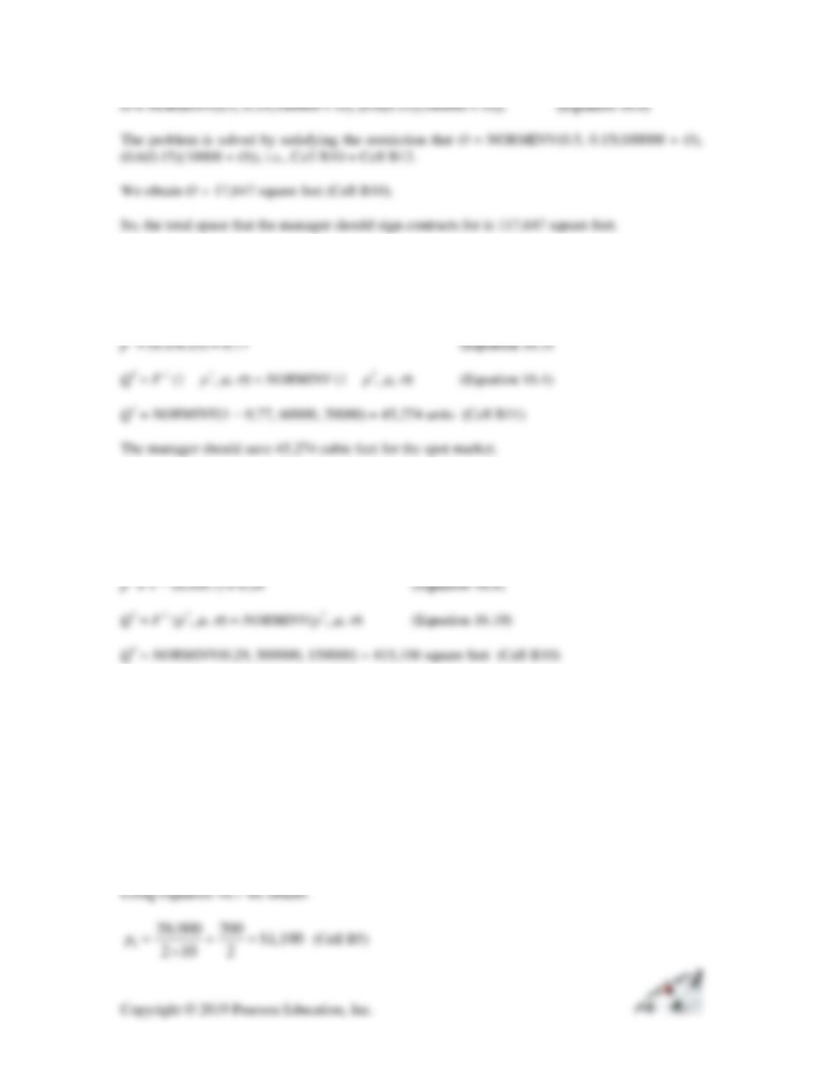
O = NORMINV(0.5, 0.15(100000 + O), (0.6(0.15)(100000 + O)). (Equation 16.8)
The problem is solved by satisfying the restriction that O = NORMINV(0.5, 0.15(100000 + O),
(0.6(0.15)(10000 + O)), i.e., Cell B10 = Cell B12.
We obtain O = 17,647 square feet (Cell B10).
So, the total space that the manager should sign contracts for is 117,647 square feet.
4. Worksheet 16-4 presents this solution:
The amount of trucking capacity the manager should save for the spot market is given by:
5. Worksheet 16-5 presents this solution.
The size of the annual contract the manager should sign is given by:
6. See spreadsheet 16-6.
Unconstrained case (See worksheet Unconstrained capacity):
Decision variables:
p1 = price that NatBike should charge customized segment
p2 = price that NatBike should charge standard segment
1
2 10 2
3
2
40,000 200 $766.67
2 30 2
p= + =
(Cell B6)
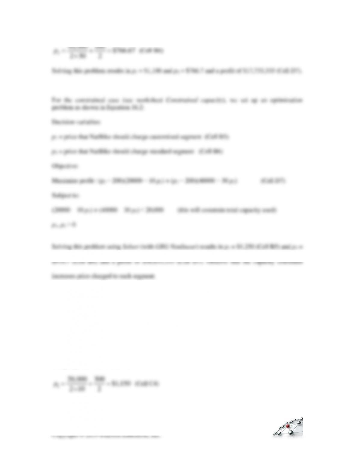
Solving this problem results in p1 = $1,100 and p2 = $766.7 and a profit of $17,733,333 (Cell D7).
For the constrained case (see worksheet Constrained capacity), we set up an optimization
problem as shown in Equation 16.2:
Decision variables:
p1 = price that NatBike should charge customized segment (Cell B5)
p2 = price that NatBike should charge standard segment (Cell B6)
Objective:
Maximize profit : (p1 − 200)(20000 − 10 p1) + (p2 − 200)(40000 − 30 p2) (Cell D7)
Subject to:
(20000 − 10 p1) + (40000 − 30 p2) ≤ 20,000 (this will constrain total capacity used)
p1, p2 ≥ 0
Solving this problem using Solver (with GRG Nonlinear) results in p1 = $1,250 (Cell B5) and p2 =
$916.7 (Cell B6) and a profit of $16,833,333 (Cell D7). Observe that the capacity constraint
increases price charged to each segment.
7. Worksheet 16-7 presents the solution to this problem.
The only change that we make (relative to 16-6) here is with respect to the production costs as
shown in bold.
Unconstrained case (see worksheet Unconstrained capacity):
Using Equation 16.1 we obtain:
1
20,000 300 $1,150
2 10 2
p= + =
(Cell C4)
4
2
40,000 200 $766.67
2 30 2
p= + =
(Cell C5)
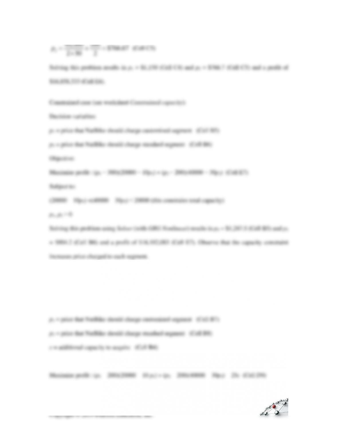
Solving this problem results in p1 = $1,150 (Cell C4) and p2 = $766.7 (Cell C5) and a profit of
$16,858,333 (Cell E6).
Constrained case (see worksheet Constrained capacity):
Decision variables:
p1 = price that NatBike should charge customized segment (Cell B5)
p2 = price that NatBike should charge standard segment (Cell B6)
Objective:
Maximize profit : (p1 − 300)(20000 − 10p1) + (p2 − 200)(40000 − 30p2) (Cell E7)
Subject to:
(20000 − 10p1) +(40000 − 30p2) ≤ 20000 (this constrains total capacity)
p1, p2 ≥ 0
Solving this problem using Solver (with GRG Nonlinear) results in p1 = $1,287.5 (Cell B5) and p2
= $904.2 (Cell B6) and a profit of $16,102,083 (Cell E7). Observe that the capacity constraint
increases price charged to each segment.
8. Worksheet 16-8 presents the solution to this problem.
In this case we allow for acquiring additional capacity at a cost
Decision variables:
Objective:
Subject to:
5
Observe that even though additional capacity is more expensive than regular capacity, it is
9. Worksheet 16-9 presents the solution to this problem:
Fixed price model (See worksheet Fixed price):
Decision variables:
Objective:
Subject to:
6
Objective:
Quantity model (see worksheet Quantity):
Decision variables:
Objective:
7
p1, p2, p3, q ≥ 0