Chapter 9: Sales and Operations Planning
We define a comprehensive set of decision variables that are utilized in Exercises 9-1–9-
3 depending on the problem context.
Decision Variables:
Exercise 9-1:
Minimize
====
+++
12
1
12
1
12
1
12
1
403222400
it
it
it
ttPIOW
Subject to:
Workforce constraints:
(a) Spreadsheet Exercise 9-1 provides the solution to this problem and the corresponding
aggregate plan. On worksheet Planning set Cell C39 to 0 (no promotion) and run Solver.
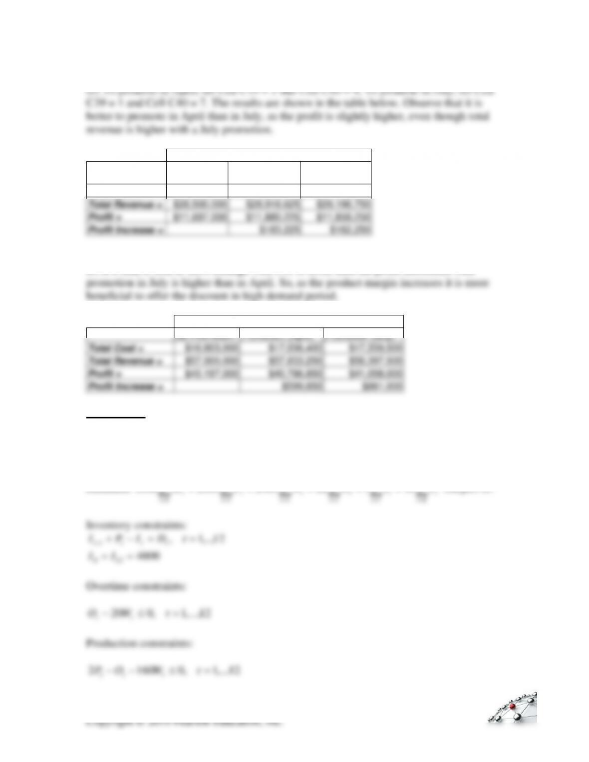
Price=$125
Total Cost
No Promotion
Promotion
(April)
Promotion
(July)
Total Cost =
$16,803,000
$17,036,400
$17,339,500
Total Revenue =
$28,500,000
$28,916,625
$29,198,750
Profit =
$11,697,000
$11,880,225
$11,859,250
Profit Increase =
$183,225
$162,250
(c) If a sink is sold at $250 (change Cell C41 to 250), then the profit associated with
Price= $250
Total Cost
No Promotion
Promotion (April)
Promotion (July)
Total Cost =
$16,803,000
$17,036,400
$17,339,500
Total Revenue =
$57,000,000
$57,833,250
$58,397,500
Profit =
$40,197,000
$40,796,850
$41,058,000
Profit Increase =
$599,850
$861,000
Exercise 9-2:
We now include hiring and layoff costs in the model. Note that the workforce level
constraints also change.
Minimize
======
+++++
12
1
12
1
12
1
12
1
12
1
12
1
40322240020001000
it
it
it
tt
tt
ttPIOWFH
Subject to:
Workforce constraints:
0=W
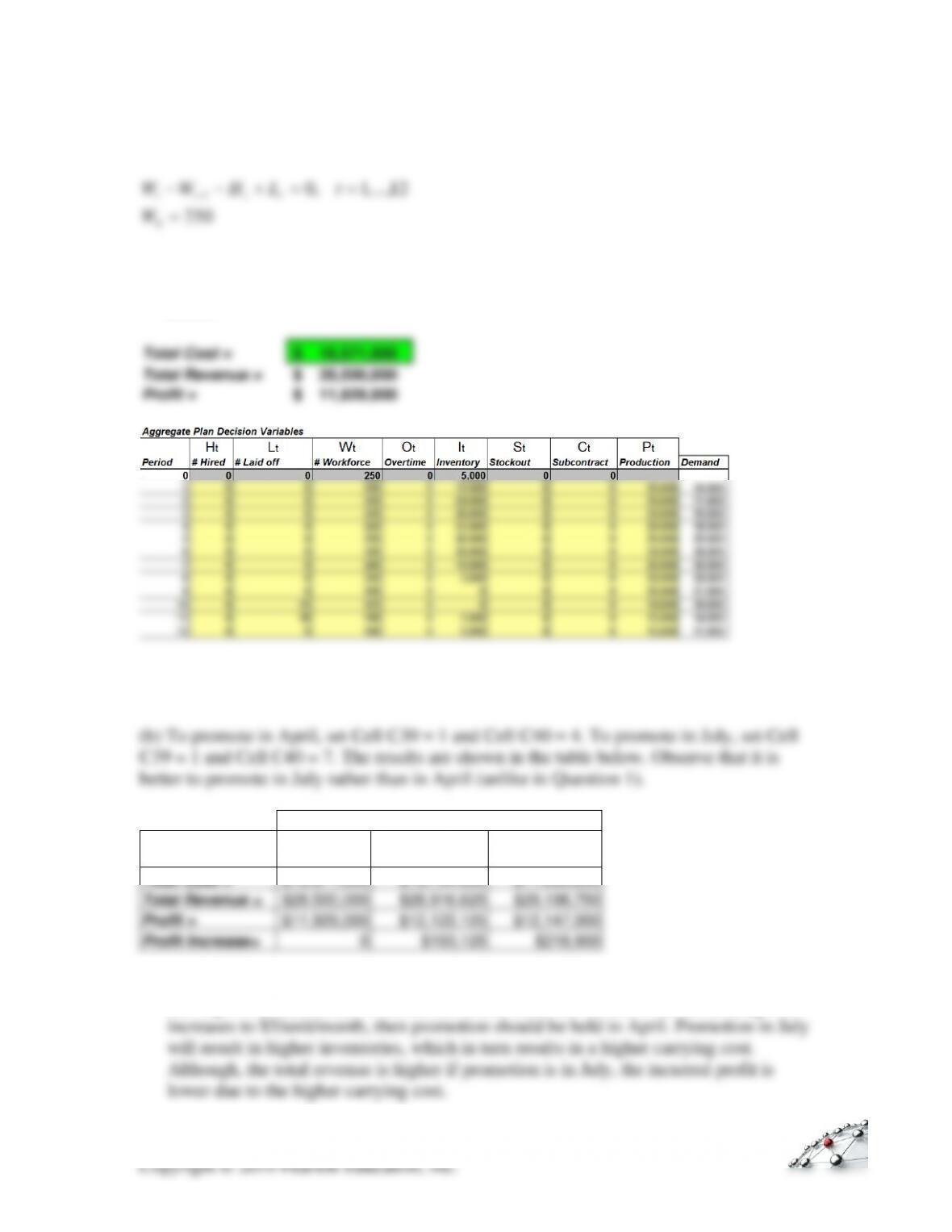
(a) Spreadsheet Exercise 9-2 provides the solution to this problem and the corresponding
aggregate plan. On worksheet Planning set Cell C39 to 0 (no promotion) and run
Solver.
Total Cost =
$ 16,571,000
Total Revenue =
$ 28,500,000
Profit =
$ 11,929,000
Some layoffs occur in months 10 and 11 under this plan, resulting in the somewhat higher
profits than 1(a).
Total Cost
No
Promotion
Promotion
(April)
Promotion
(July)
Total Cost =
$16,571,000
$16,794,500
$17,050,850
Total Revenue =
$28,500,000
$28,916,625
$29,198,750
Profit =
$11,929,000
$12,122,125
$12,147,900
Profit Increase=
0
$193,125
$218,900
(c) To increase holding cost to $5, change Cell E7 in worksheet Data to 5. Now repeat
the steps from (a) and (b) to obtain the results table shown below. If the holding cost
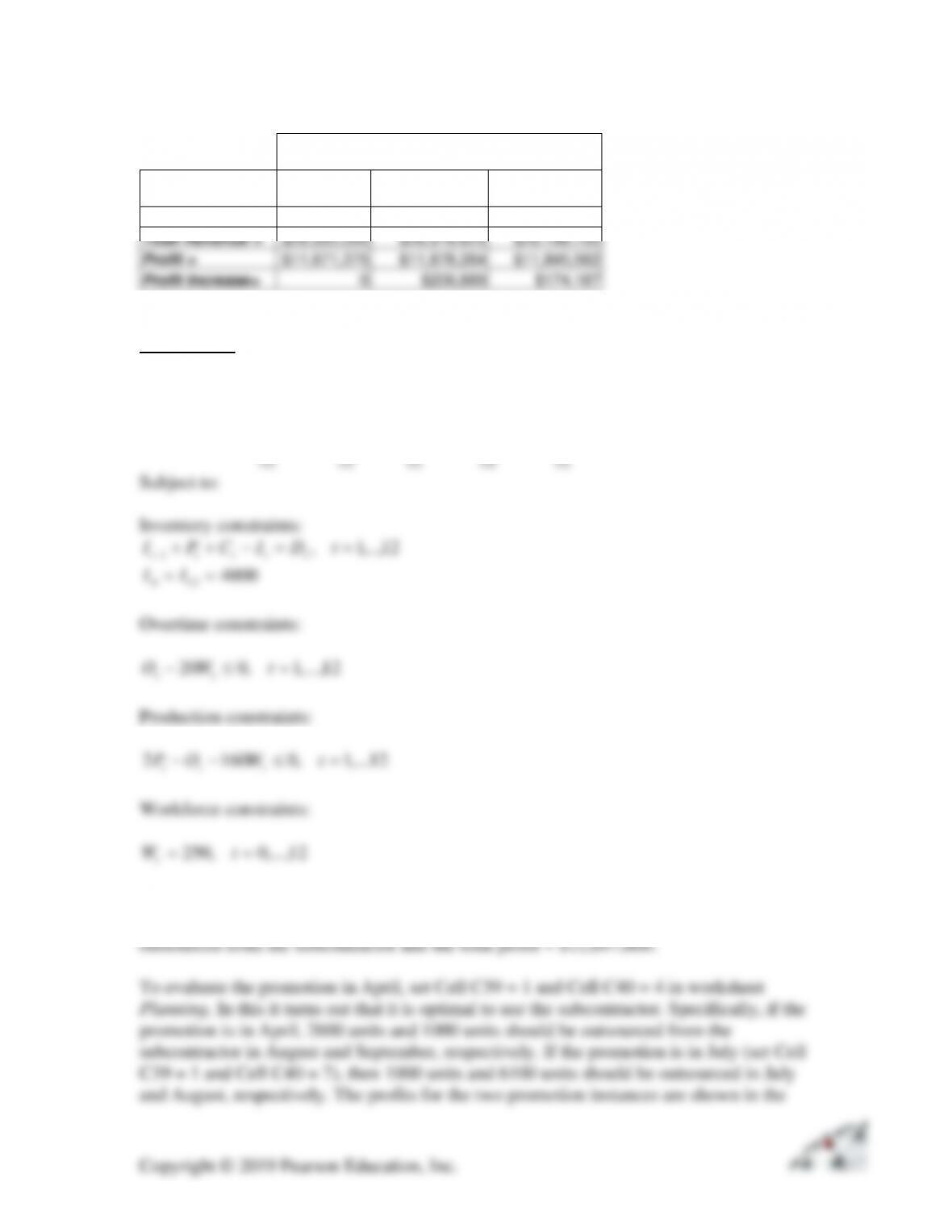
Holding =
$5/unit/month
Total Cost
No
Promotion
Promotion
(April)
Promotion
(July)
Total Cost =
$16,828,625
$17,038,361
$17,353,188
Total Revenue =
$28,500,000
$28,916,625
$29,198,750
Profit =
$11,671,375
$11,878,264
$11,845,562
Profit Increase=
0
$206,889
$174,187
Exercise 9-3:
In this case, we add the subcontract option to problem information given in 9-1
Minimize
=====
++++
12
1
12
1
12
1
12
1
12
1
74403222400
it
it
it
it
ttCPIOW
Use spreadsheet Exercise 9-3 for the analysis. To evaluate the case without promotion,
set Cell C39 =0 in worksheet Planning. In the absence of a promotion, no units are
Copyright © 2019 Pearson Education, Inc.
table below. The need for subcontracting arises because promotion induces additional
demand during certain months, which will not be cost effective for Lavare to produce by
itself, as the carrying cost will outweigh the costs paid to the subcontractor.
Total Cost
Promotion
(April)
Promotion
(July)
Total Cost =
$17,000,100
$17,251,400
Total Revenue =
$28,916,625
$29,198,750
Profit =
$11,916,525
$11,947,350
Problems 9-4 ~ 9-6
We define a comprehensive set of decision variables that are utilized in Problems 9-4–9-6
depending on the problem context.
Decision Variables:
Parameters:
Exercise 9-4:
Minimize
====
+++
12
1
12
1
12
1
12
1
354151600
it
it
it
ttPIOW
Subject to:
Production constraints:
12,…1,01602=−− tWOP ttt
Workforce constraints:
12,…,0,250 == tWt
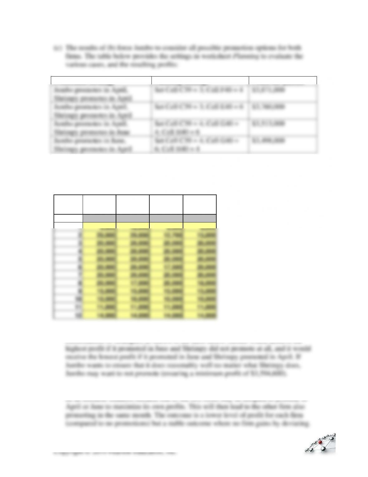
(a) All analysis is done using spreadsheet Exercise 9-4. For the case where there is no
promotion by either Jumbo or Shrimpy, we set Cell C39 = 0 in worksheet Planning. Run
Solver to obtain the following results.
Copyright © 2019 Pearson Education, Inc.
(c) The results of (b) force Jumbo to consider all possible promotion options for both
firms. The table below provides the settings in worksheet Planning to evaluate the
various cases, and the resulting profits:
Promotion Strategy
Planning Settings
Profit for Jumbo
Jumbo promotes in April,
Shrimpy promotes in April
Set Cell C39 = 3; Cell F40 = 4
$3,871,000
Jumbo promotes in April,
Shrimpy promotes in April
Set Cell C39 = 3; Cell E40 = 6
$3,760,000
Jumbo promotes in April,
Shrimpy promotes in June
Set Cell C39 = 4; Cell G40 =
4; Cell H40 = 6
$3,513,000
Jumbo promotes in June,
Shrimpy promotes in April
Set Cell C39 = 4; Cell G40 =
6; Cell H40 = 4
$3,498,000
The production plan is shown as follows for each case (first digit represents the month
that Jumbo promotes and second digit the month that Shrimpy promotes):
44
66
46
64
Period
Production
Production
Production
Production
0
1
9,000
12,000
8,000
8,000
2
20,000
20,000
12,700
15,000
3
20,000
20,000
20,000
20,000
4
20,000
20,000
20,000
20,000
5
20,000
20,000
20,000
20,000
6
20,000
20,000
17,500
20,000
7
20,000
20,000
20,000
20,000
8
20,000
17,000
20,000
18,000
9
15,000
15,000
15,000
15,000
10
10,000
10,000
10,000
10,000
11
11,000
11,000
11,000
11,000
12
14,000
14,000
14,000
14,000
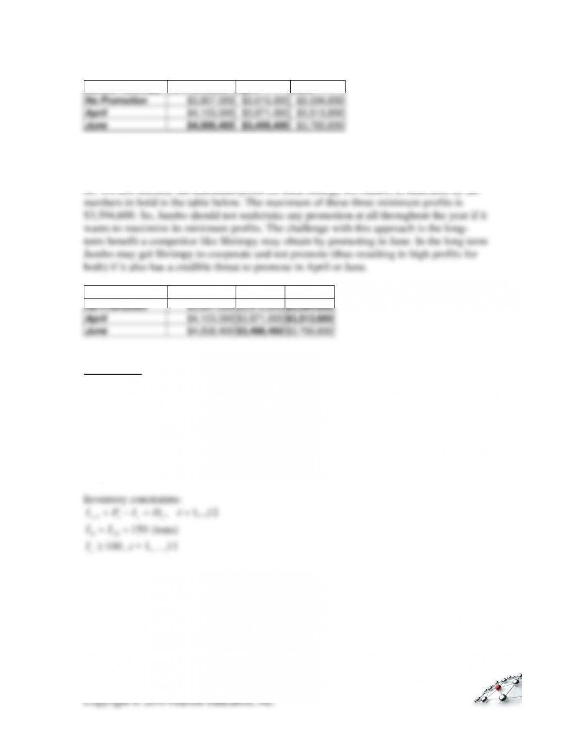
(d) There are three strategies for both Jumbo and Shrimpy, which leads to a total of 9
combinations of strategies, as shown in the table below. Jumbo would achieve the
Profits for both firms are higher if neither firm promotes. This is, however, likely to
Jumbo \ Shrimpy
No Promotion
April
June
No Promotion
$3,907,000
$3,615,000
$3,594,600
April
$4,103,000
$3,871,000
$3,513,800
June
$4,008,400
$3,498,400
$3,760,600
Note: number in each cell represents Jumbo’s profit
(e) We first identify the minimum profit for each strategy for Jumbo, as indicated by the
Jumbo \ Shrimpy
No Promotion
April
June
No Promotion
$3,907,000
$3,615,000
$3,594,600
April
$4,103,000
$3,871,000
$3,513,800
June
$4,008,400
$3,498,400
$3,760,600
Exercise 9-5:
Re-define two variables:
t
W
: workforce, in terms of # of shifts (per shift= 100 employees)
t
O
: overtime (hours per shift)
Minimize
====
+++
12
1
12
1
12
1
12
1
1000100100*151000*160
it
it
it
ttPIOW
Subject to:
Copyright © 2019 Pearson Education, Inc.
Overtime constraints:
12,…,1,020 =− tWO tt
Production constraints:
12,...1,0160 =−− tWOP ttt
Workforce constraints:
12,…,0,2 == tWt
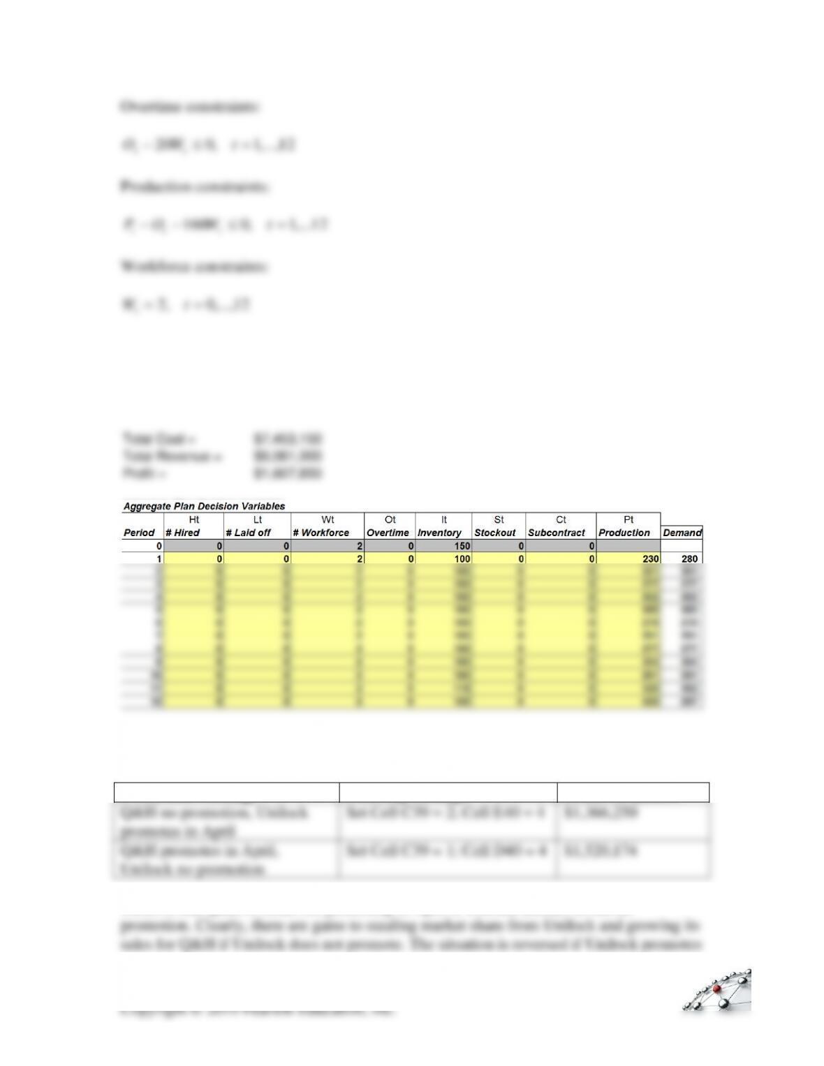
(a) We use the spreadsheet Exercise 9-5 for the analysis. We assume that the
workforce size stays unchanged but the number of overtime hours worked can
vary from one month to another. For the case with no promotion, enter Cell C39 =
0 and run Solver on worksheet Planning to obtain the following results:
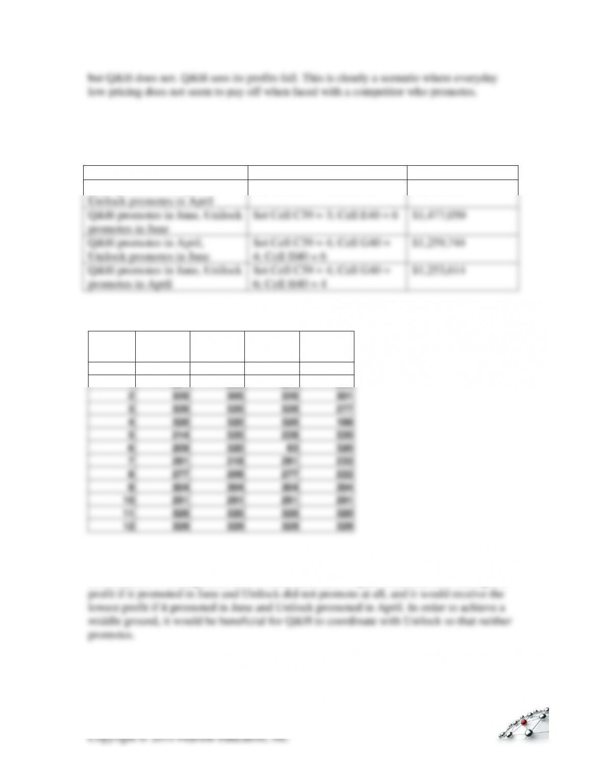
(b) The table below provides the settings in worksheet Planning to evaluate the two cases,
and the resulting profits:
Promotion Strategy
Planning Settings
Profit for Jumbo
Q&H no promotion, Unilock
promotes in April
Set Cell C39 = 2; Cell E40 = 4
$1,366,250
Q&H promotes in April,
Unilock no promotion
Set Cell C39 = 1; Cell D40 = 4
$1,520,174
Observe that Q&H is better off promoting in April if Unilock decides to run no
Copyright © 2019 Pearson Education, Inc.
but Q&H does not. Q&H sees its profits fall. This is clearly a scenario where everyday
low pricing does not seem to pay off when faced with a competitor who promotes.
(c) The results of (b) force Q&H to consider all possible promotion options for both
firms. The table below provides the settings in worksheet Planning to evaluate the
two cases, and the resulting profits:
Promotion Strategy
Planning Settings
Profit for Q&H
Q&H promotes in April,
Unilock promotes in April
Set Cell C39 = 3; Cell F40 = 4
$1,466,410
Q&H promotes in June, Unilock
promotes in June
Set Cell C39 = 3; Cell E40 = 6
$1,477,050
Q&H promotes in April,
Unilock promotes in June
Set Cell C39 = 4; Cell G40 =
4; Cell H40 = 6
$1,259,744
Q&H promotes in June, Unilock
promotes in April
Set Cell C39 = 4; Cell G40 =
6; Cell H40 = 4
$1,253,614
The production plan in each case is shown as follows:
44
66
46
64
Period
Production
Production
Production
Production
0
1
291
230
263
230
2
320
305
320
301
3
320
320
320
277
4
320
320
320
188
5
214
320
228
320
6
209
320
83
320
7
291
218
291
233
8
277
208
277
222
9
304
304
304
304
10
291
291
291
291
11
320
320
320
320
12
329
329
329
329
(d) There are three strategies for both Q&H and Unilock, which leads to a total of nine
combinations of strategies, as shown in the table below. Q&H would achieve the highest
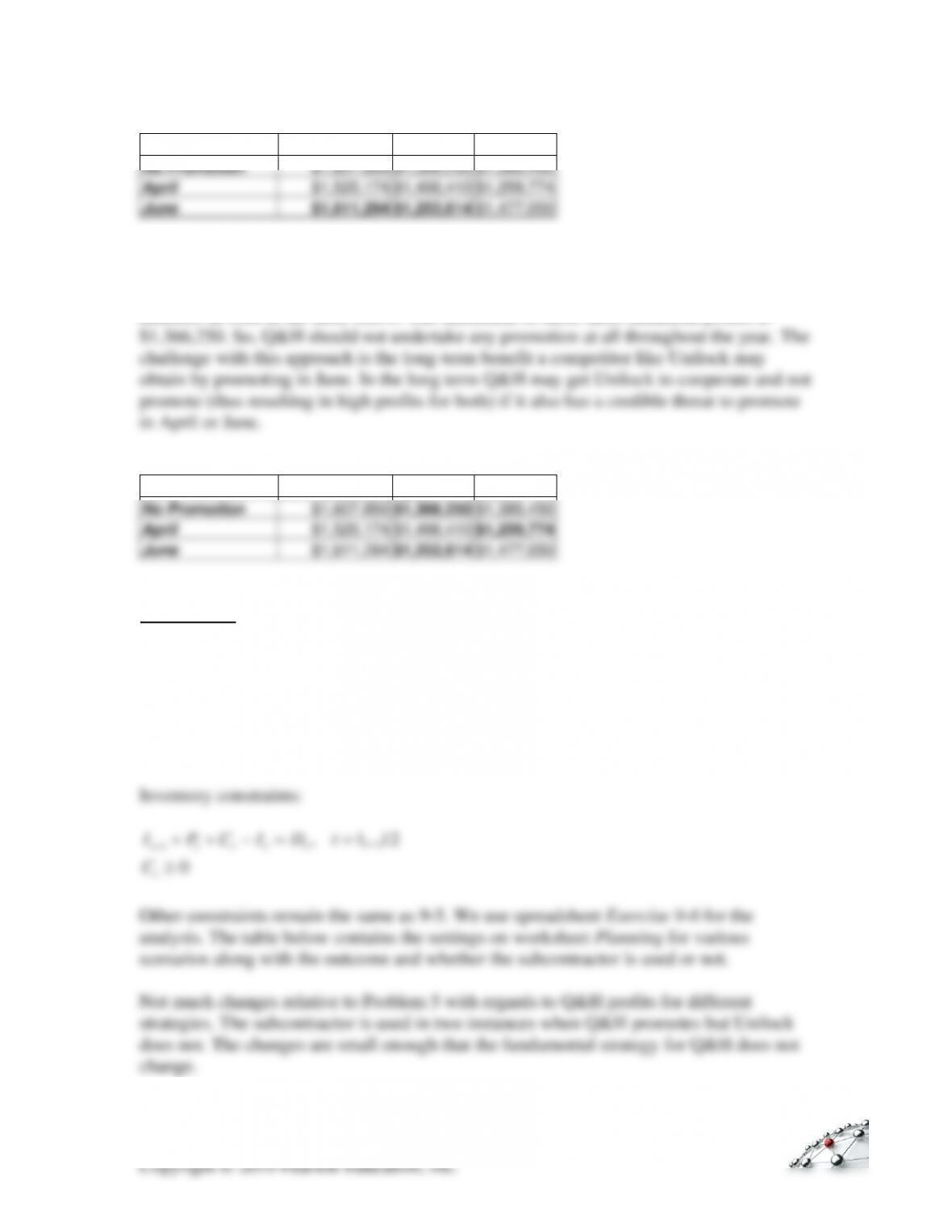
Q&H \ Unilock
No Promotion
April
June
No Promotion
$1,607,850
$1,366,250
$1,385,450
April
$1,520,174
$1,466,410
$1,259,774
June
$1,611,294
$1,253,614
$1,477,050
Note: number in each cell represents Q&H’s profit
(e) We first identify the minimum profit for each strategy for Q&H, as indicated by the
numbers in bold in the table below. The maximum of these three minimum profits is
Q&H \ Unilock
No Promotion
April
June
No Promotion
$1,607,850
$1,366,250
$1,385,450
April
$1,520,174
$1,466,410
$1,259,774
June
$1,611,294
$1,253,614
$1,477,050
Exercise 9-6:
Part of the formulation needs to be revised to allow for subcontracting.
Minimize
=====
++++
12
1
12
1
12
1
12
1
12
1
23001000100100*151000*160
it
it
it
it
ttCPIOW
Subject to:
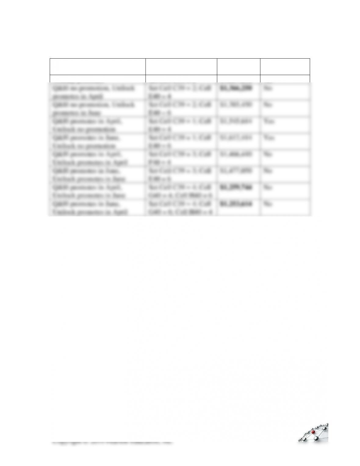
Promotion Strategy
Planning Settings
Profit for
Q&H
Subcontractor
Used?
Nobody promotes
Set Cell C39 = 0
$1,607,850
No
Q&H no promotion, Unilock
promotes in April
Set Cell C39 = 2; Cell
E40 = 4
$1,366,250
No
Q&H no promotion, Unilock
promotes in June
Set Cell C39 = 2; Cell
E40 = 6
$1,385,450
No
Q&H promotes in April,
Unilock no promotion
Set Cell C39 = 1; Cell
E40 = 4
$1,545,614
Yes
Q&H promotes in June,
Unilock no promotion
Set Cell C39 = 1; Cell
E40 = 6
$1,612,414
Yes
Q&H promotes in April,
Unilock promotes in April
Set Cell C39 = 3; Cell
F40 = 4
$1,466,410
No
Q&H promotes in June,
Unilock promotes in June
Set Cell C39 = 3; Cell
E40 = 6
$1,477,050
No
Q&H promotes in April,
Unilock promotes in June
Set Cell C39 = 4; Cell
G40 = 4; Cell H40 = 6
$1,259,744
No
Q&H promotes in June,
Unilock promotes in April
Set Cell C39 = 4; Cell
G40 = 6; Cell H40 = 4
$1,253,614
No