12
16. Excel Worksheet Ex 12–16 illustrates these computations.
(a)
Disaggregated Option:
From the previous problem, we know that the total ss for Europe is 48,384 (Cell C41)
Aggregated Option:
(c) If the lead time changes to four weeks, we evaluate the safety stocks and associated costs in a
similar manner.
The holding cost from the disaggregated option = (200)(0.25)(34213) = $1,710,650 (Cell F42)
17. Excel Worksheet Ex 12–17 illustrates these computations.
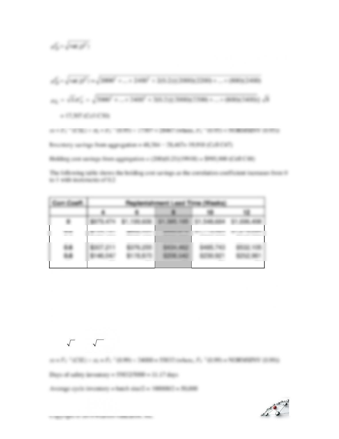
Since the demand at various locations is not independent, we utilize the following expressions for
the aggregated option:
k
= ji
ji
ij
ii
1
)var( DC
C
D=
For
= 0.2 (set Cell C18 = 0.2)
14
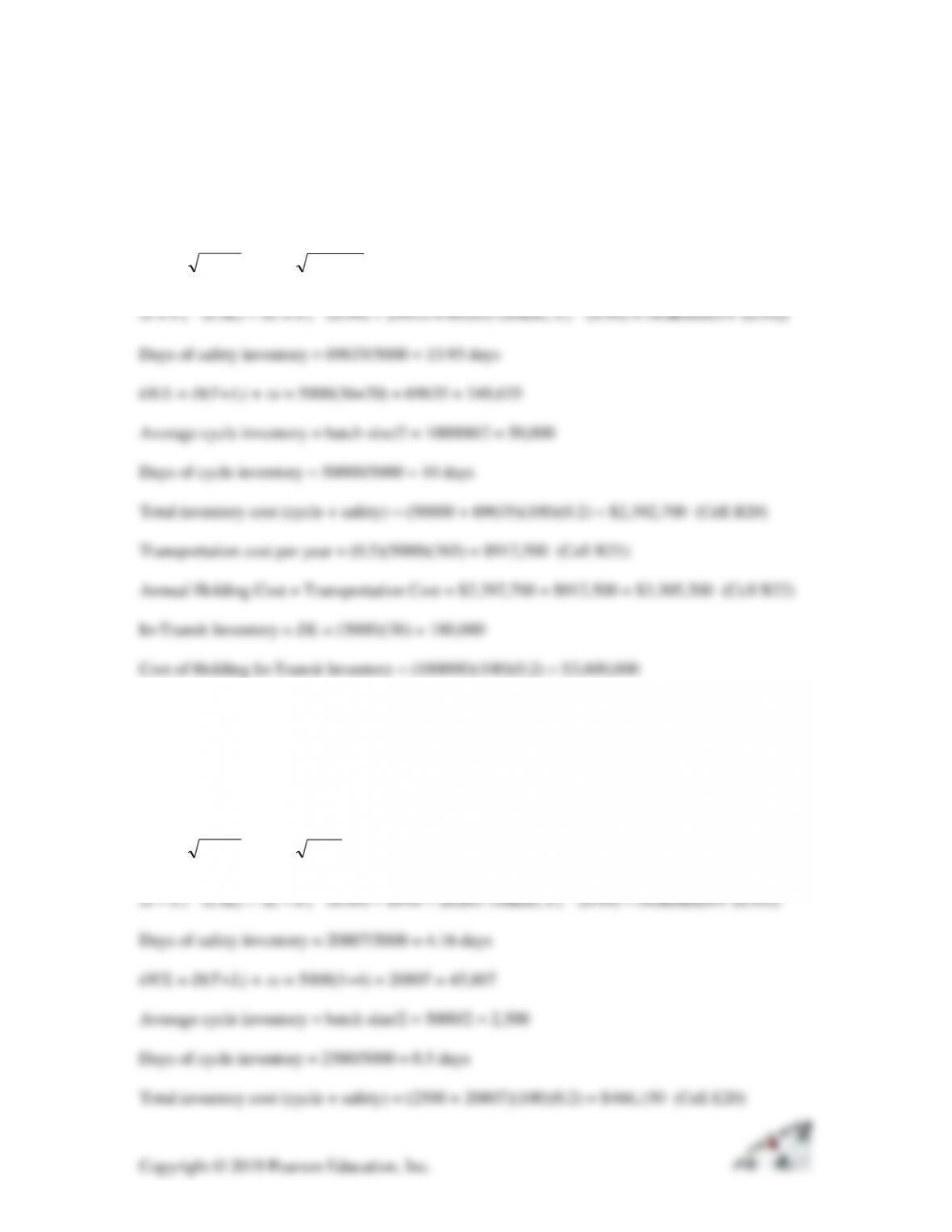
Days of cycle inventory = 50000/5000 = 10 days
In-Transit Inventory = DL = (5000)(36) = 180,000
Using Air Transportation:
Average batch size = DT = (5000)(1) = 5,000
L
=
D
L
=
)4000(4
= 8,000
−1 (CSL)
−1 (0.99) 8000 = 18,611 (where, FS
−1 (0.99) = NORMSINV (0.99))
15
20. Excel worksheet 12-20 illustrates these computations.
16
21. Excel Worksheet Ex 12–21 illustrates these computations.
Using Sea Transportation:
Average batch size = DT = (5000)(20) = 100,000
L
=
D
TL +
=
)4000(2036 +
= 29,933
−1 (CSL)
−1 (0.99) 29933 = 69,635 (where, FS
−1 (0.99) = NORMSINV (0.99))
Total Costs (including in-transit inventory) = $3,029,140 + $3,600,000 = $6,905,200 (Cell B25)
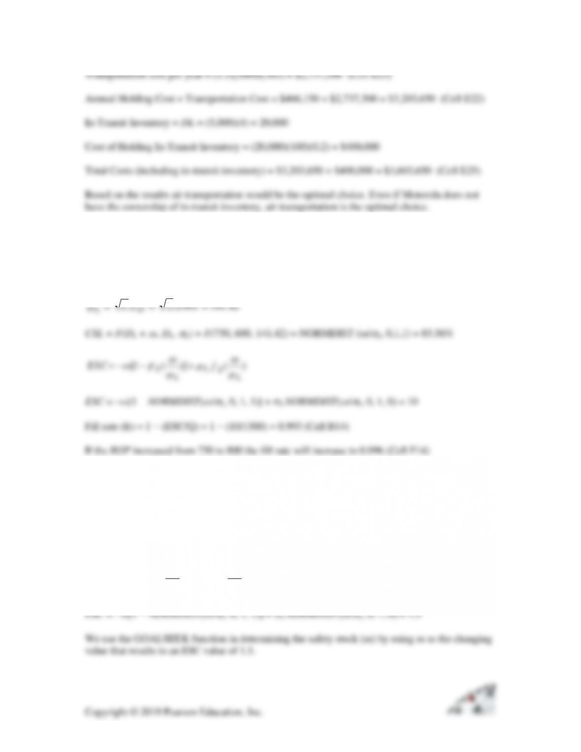
Using Air Transportation:
Average batch size = DT = (5000)(1) = 5,000
L
=
D
TL +
=
)4000(14 +
= 8,944
−1 (CSL)
−1 (0.99) 8944 = 20,807 (where, FS
−1 (0.99) = NORMSINV (0.99))
Copyright © 2019 Pearson Education, Inc.
17
Transportation cost per year = (1.5)(5000)(365) = $2,737,500 (Cell E21)
Annual Holding Cost + Transportation Cost = $466,150 + $2,737,500 = $3,203,650 (Cell E22)
In-Transit Inventory = DL = (5,000)(4) = 20,000
Cost of Holding In-Transit Inventory = (20,000)(100)(0.2) = $400,000
Total Costs (including in-transit inventory) = $3,203,650 + $400,000 = $3,603,650 (Cell E25)
Based on the results air transportation would be the optimal choice. Even if Motorola does not
have the ownership of in-transit inventory, air transportation is the optimal choice.
22. Excel Worksheet Ex 12–22 illustrates these computations.
ss = ROP − DL = 750 – 300(2) = 750 − 600 = 150
L
=
D
L
=
)100(2
= 141.42
CSL = F(DL + ss, DL,
L) = F(750, 600, 141.42) = NORMDIST (ss/
L, 0,1,1) = 85.56%
)()](1[
L
S
L
L
S
ss
f
ss
F
ssESC +−−=
ESC = –ss[1 − NORMDIST(ss/
L, 0, 1, 1)] + L NORMDIST(ss/
L, 0, 1, 0) = 10
Fill rate (fr) = 1 − (ESC/Q) = 1 − (10/1500) = 0.993 (Cell B14)
If the ROP increased from 750 to 800 the fill rate will increase to 0.996 (Cell F14)
23. Excel Worksheet Ex 12–23 illustrates these computations.
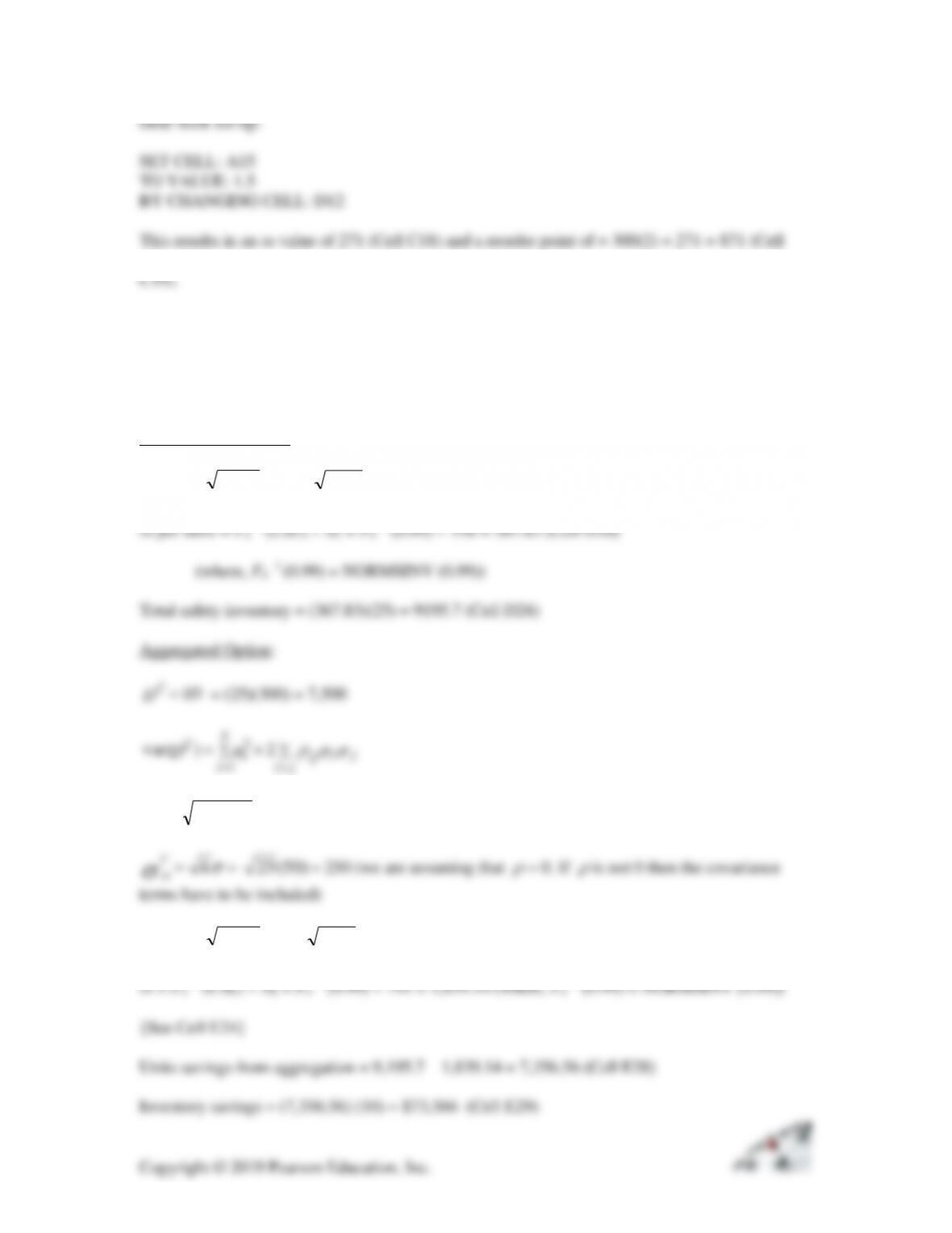
Fill rate (fr) = 1 − (ESC/1500) = 0.999
So, ESC = 1.5
)()](1[
L
S
L
L
S
ss
f
ss
F
ssESC +−−=
]
Copyright © 2019 Pearson Education, Inc.
18
Goal Seek set-up:
SET CELL: A15
TO VALUE: 1.5
BY CHANGING CELL: D12
This results in an ss value of 271 (Cell C18) and a reorder point of = 300(2) + 271 = 871 (Cell
C19).
24. Excel Worksheet Ex 12–24 illustrates these computations.
(a) (see worksheet 12.24 (a))
Disaggregated Option:
TL+
=
D
TL +
=
)50(73 +
= 158
−1 (CSL)
−1 (0.99) 158 = 367.83 (Cell D20)
−1 (0.99) = NORMSINV (0.99))
= ji
ji
ij
ii
1
)var( DC
C
D=
k
C
D=
=
)50(25
= 250 (we are assuming that
= 0. If
is not 0 then the covariance
terms have to be included)
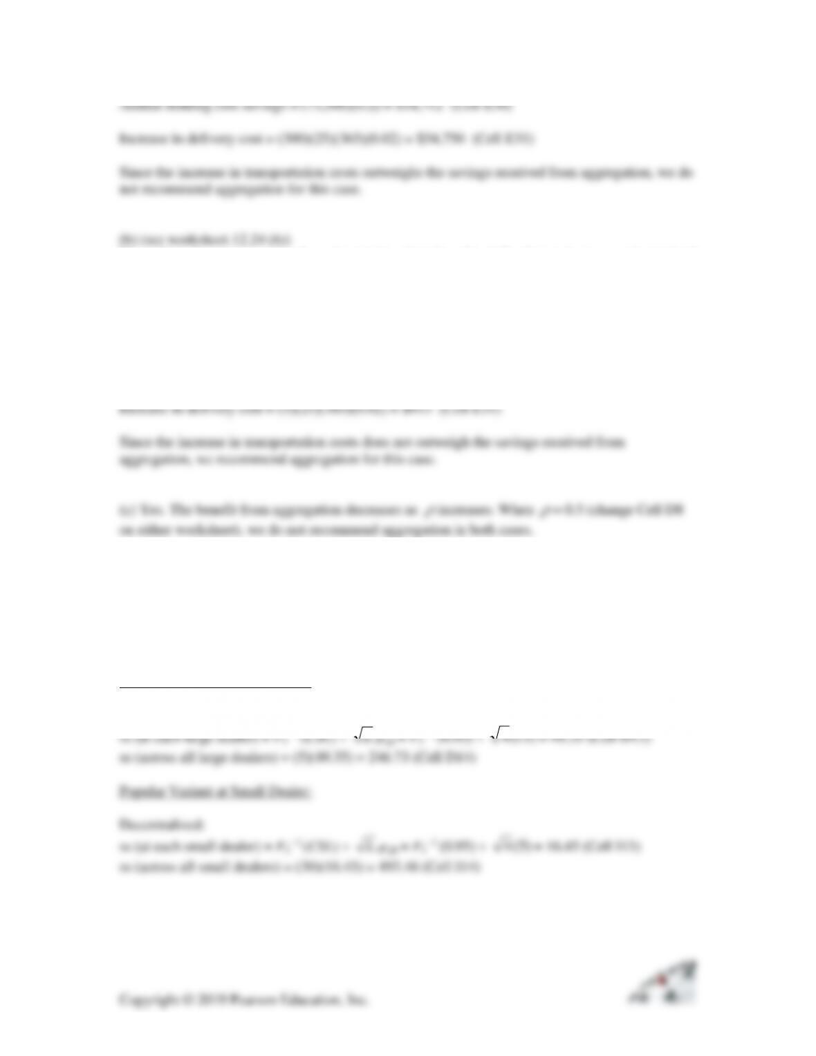
TL+
=
C
D
TL
+
=
)250(73 +
= 791
−1 (CSL)
−1 (0.99) 791 = 1,839.14 (where, FS
−1 (0.99) = NORMSINV (0.99))
Copyright © 2019 Pearson Education, Inc.
19
Annual holding cost savings = (73,566)(0.2) = $14,712 (Cell E30)
Increase in delivery cost = (300)(25)(365)(0.02) = $54,750 (Cell E31)
Since the increase in transportation costs outweighs the savings received from aggregation, we do
not recommend aggregation for this case.
(b) (see worksheet 12.24 (b))
We utilize the same approach as in (a) by changing the daily demand mean and standard
deviation to 5 and 4, respectively
Units savings from aggregation = 735.66 − 147.13 = 588.52 (Cell E28)
Inventory savings = (588.52) (10) = $ 5,885.2 (Cell E29)
Annual holding cost savings = ($5885.2)(0.2) = $1,177 (Cell E30)
25. Excel Worksheet Ex 12–25 illustrates these computations. See worksheet 12.25 (a-d) for parts
(a) – (d)
(a)
Popular Variant at Large Dealer:
Decentralized:
−1 (CSL)
−1 (0.95)
ss (across all large dealers) = (5)(49.35) = 246.73 (Cell D14)
Popular Variant at Small Dealer:
Decentralized:
ss (at each small dealer) = FS
−1 (CSL)
D
L
= FS
−1 (0.95)
)5(4
= 16.45 (Cell I13)
ss (across all small dealers) = (30)(16.45) = 493.46 (Cell I14)
Copyright © 2019 Pearson Education, Inc.
20
(b )
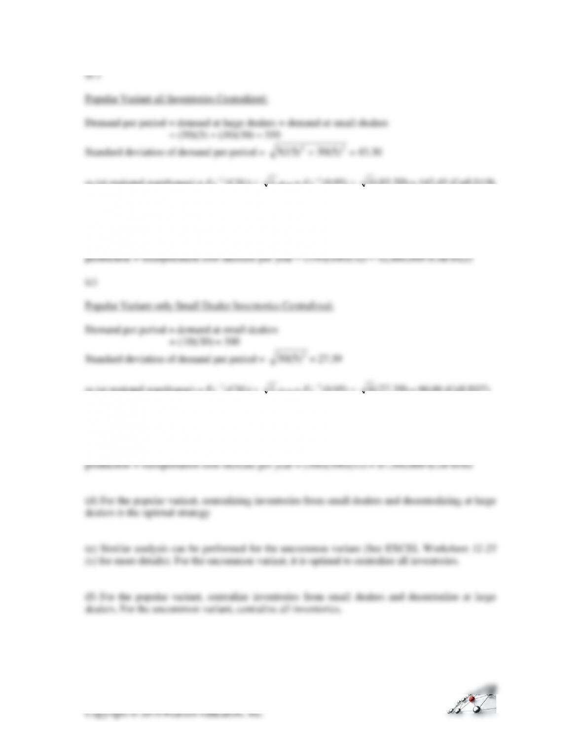
Popular Variant all Inventories Centralized:
Demand per period = demand at large dealers + demand at small dealers
= (50)(5) + (10)(30) = 550
Standard deviation of demand per period =
22 )5(30)15(5 +
= 43.30
ss (at regional warehouse) = FS
D
L
= FS
)30.43(4
= 142.45 (Cell D19)
reduction in safety inventory from complete aggregation = 246.73 + 493.46 − 142.45 = 597.74
holding cost savings per year = (597.74)(20000)(0.2) = $2,390,942.52 (Cell D21)
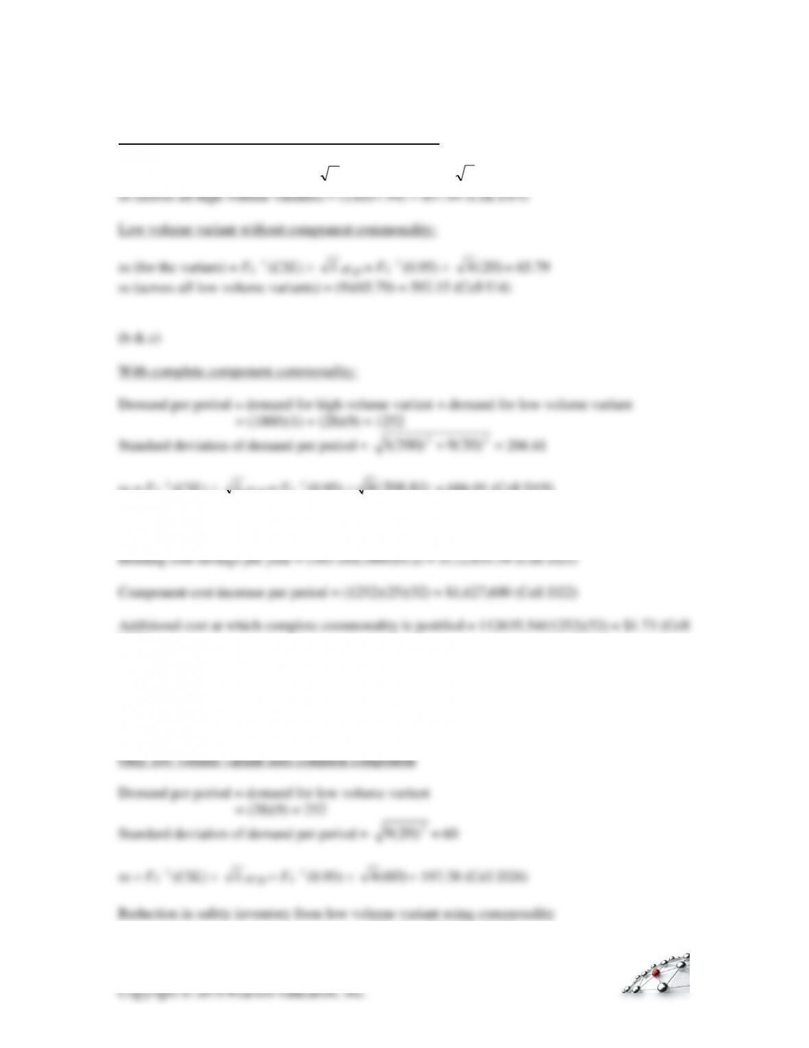
ss (at regional warehouse) = FS
D
L
= FS
)39.27(4
= 90.09 (Cell D27)
reduction in safety inventory from small dealer centralization = 493.46 − 90.09 = 403.36
holding cost savings per year = (403.36)(20000)(0.2) = $1,613,440 (Cell D29)
D
26. Excel Worksheet Ex 12–26 illustrates these computations.
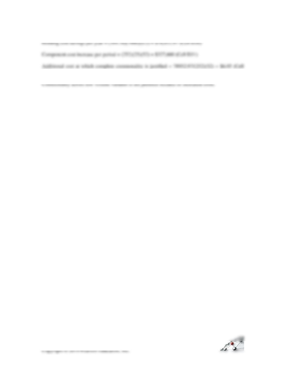
High volume variant without component commonality:
ss (for the variant) = FS
−1 (CSL)
D
L
= FS
−1 (0.95)
)200(4
= 657.94
D
L
ss = FS
D
L
= FS
4(208.81)
= 686.91 (Cell D19)
Reduction in safety inventory from complete commonality = 657.94 + 592.15 − 686.91 = 563.18
D23)
Commonality across all variants is not justified because of increased costs.
(d & e)
22
D32)