1 1 1
1
1
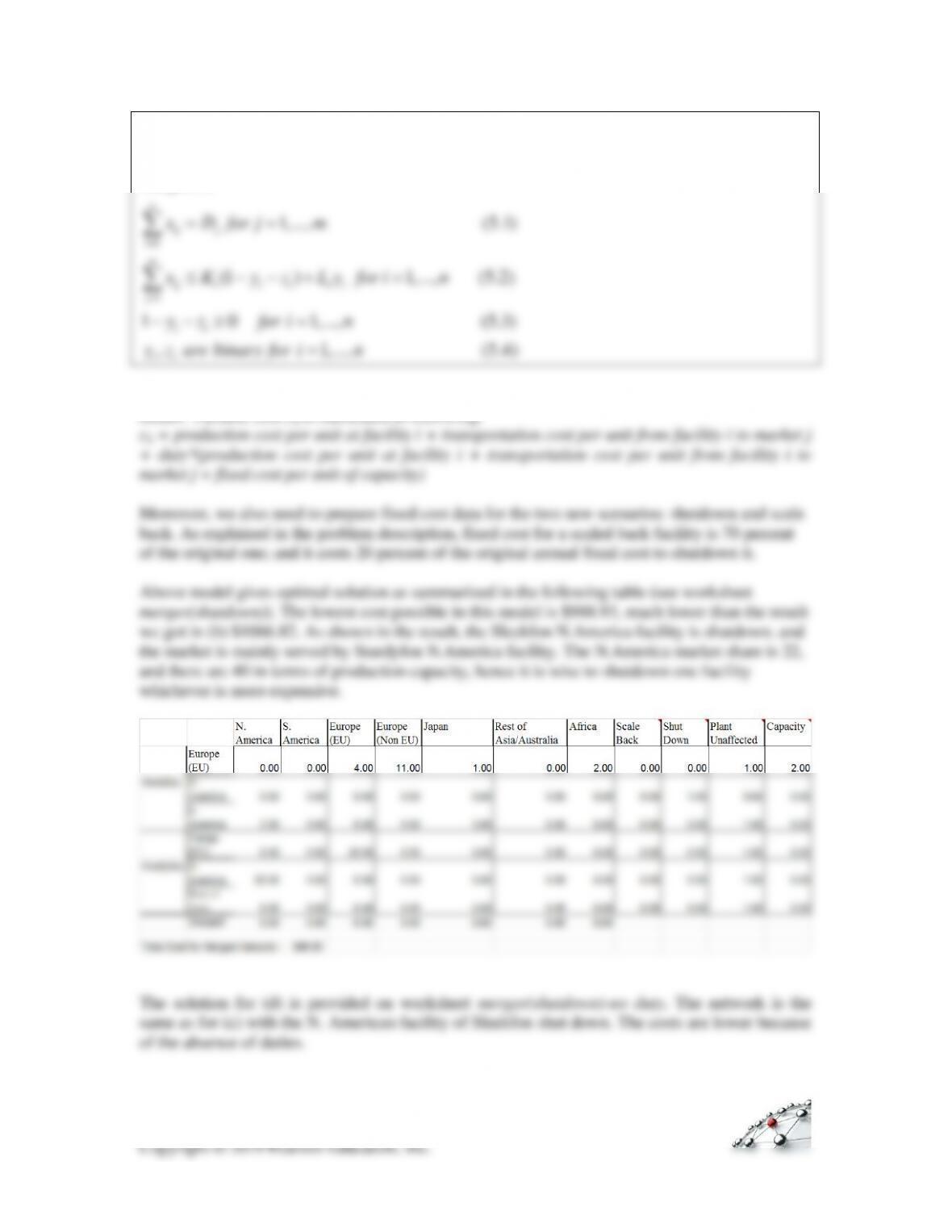
( (1 ) )
Subject to
1,…, (5.1)
(1 ) 1,…, (5.2)
1 0 1,…,
n n m
i i i i i i i ij ij
i i j
n
ij j
i
m
ij i i i i i
j
ii
Min f y z g y h z c x
x D for j m
x K y z L y for i n
y z for i n
= = =
=
=
− − + + +
==
− − + =
− − =
(5.3)
, 1,…, (5.4)
ii
y z are binary for i n=
Please note that we need to calculate the variable cost cij before we plug it into the optimization
model. Variable cost cij is calculated as following:
13
5
(a)
The model we developed in 4.d is applicable to this question. We only need to update the demand
data accordingly. Moreover, the new demand structure yields a quite different optimal
configuration of the network (see spreadsheet Exercise 5-5).
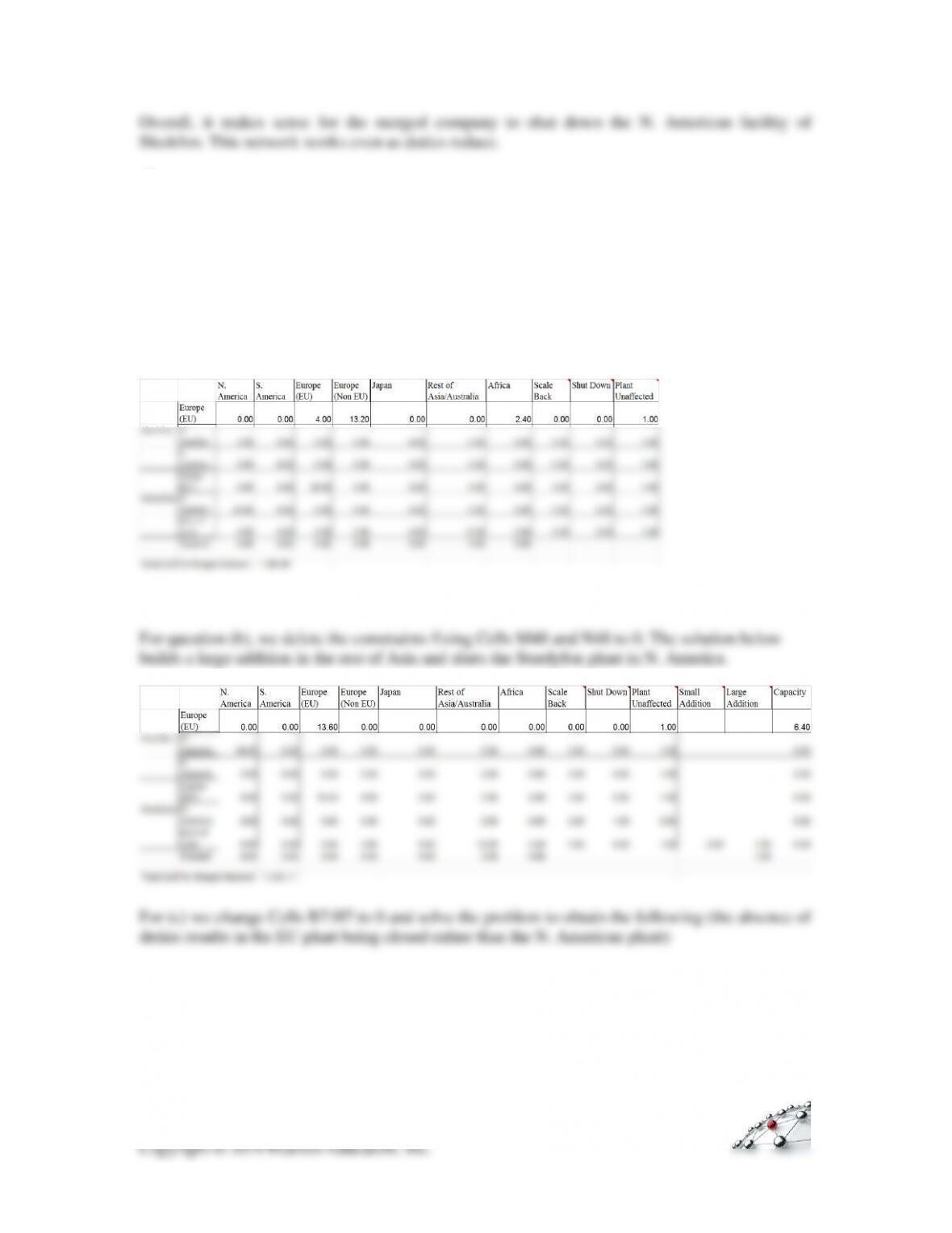
The solution for the new merged network is obtained in worksheet merger(shutdown) as shown
below (add constraints).
As shown in the table, all plants are kept open.
14
6
(a)
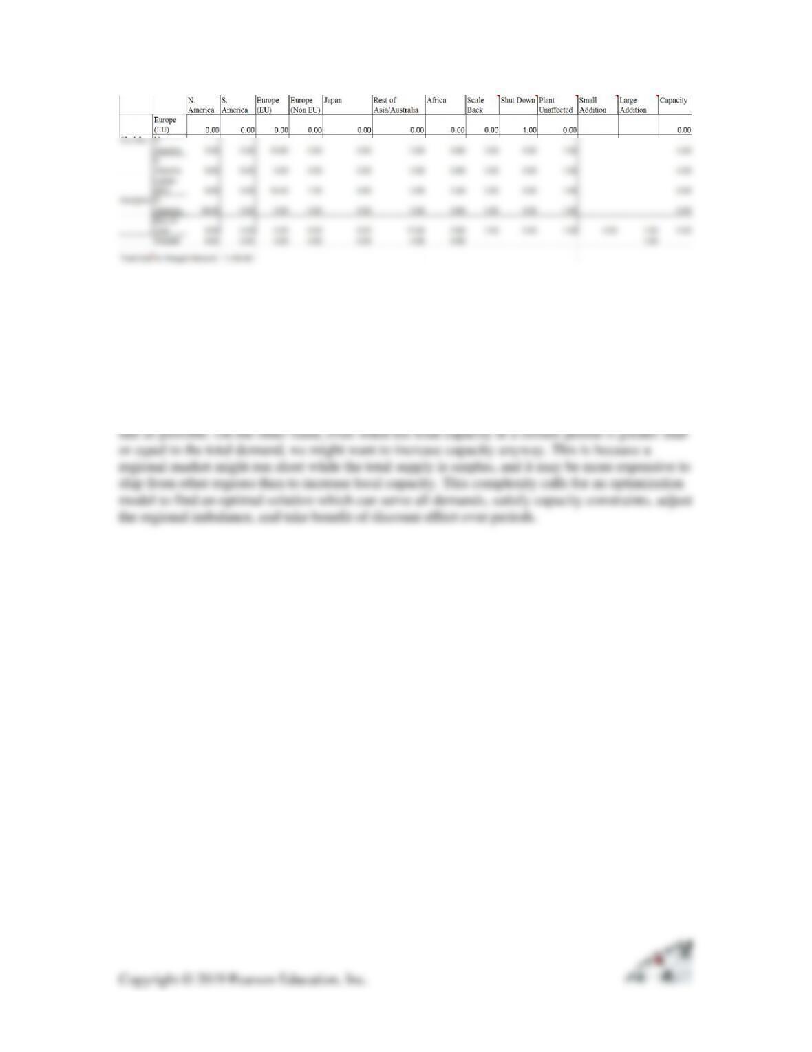
StayFresh faces a multi-period decision problem. If we treated each period separately, only two
constraints are relevant, that is, the demand and capacity constraints. Considering the multi-
period nature of this problem, it must be noted that as the demand increases steadily, we need to
add capacities eventually. However, due to the discount factor, we want to increase capacities as
jt
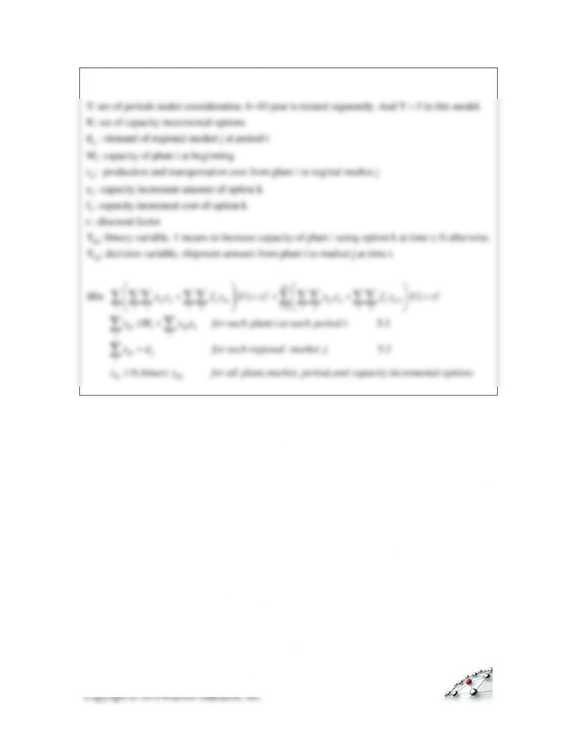
I: set of plants and potential plants
J: set of regional markets
T: set of periods under consideration. 6~10 year is treated separately. And T 5 in this model.
K: set of capacity incremental options
d
=
i
ij
k
k
: demand of regional market j at period t
M : capacity of plant i at beginning
c : production and transportation cost from plant i to reginal market j
e : capacity increment amount of option k
f : capac
ikt
ijt
ity increment cost of option k
r : discount factor
Y : binary variable. 1 means to increase capacity of plant i using option k at time t; 0 otherwise.
X : decision variable, shipment amount from plant
10
55
5
i to market j at time t
11
5.1
tt
ijt ij k ikt ij ij k ik
t i j i k t i j i k
ijt i ikt k
jt
i
Min x c f y /( r) x c f y /( r)
x M y e for each plant i at each period t
x
=
+ + + + +
+
5.2
0
jt j
i
ijt ikt
d for each regional market j
x , binary y for all plant, market, period, and capacity incremental options
=
16
SYMBOL
INPUT
CELL
jt
d
demand of regional market at period jt
B9:H9
i
M
capacity of plant at beginningi
C12:C14
ij
c
production and transportation cost from plant i to regional market j
B5:F8
k
e
capacity increment amount of option k
D12:D17
k
f
capacity increment cost of option k
C43:I45
r
discount factor
D48
ikt
Y
binary variable. 1 means to increase capacity of plant using option at time ; 0 otherwisei k t
I5:Q8
ijt
X
decision variable, shipment amount from plant to market at time i j t
B22:E25
H22:K25
N22:Q25
T22:W25
Z22:AC25
obj
objective function
C31
5.1
capacity constraint
G22:G25
M22:M25
S22:S25
Y22:Y25
Ae22:Ae25
5.2
demand constraint
B26:E26
H26:K26
N26:Q26
T26:W26
Z26:AC26
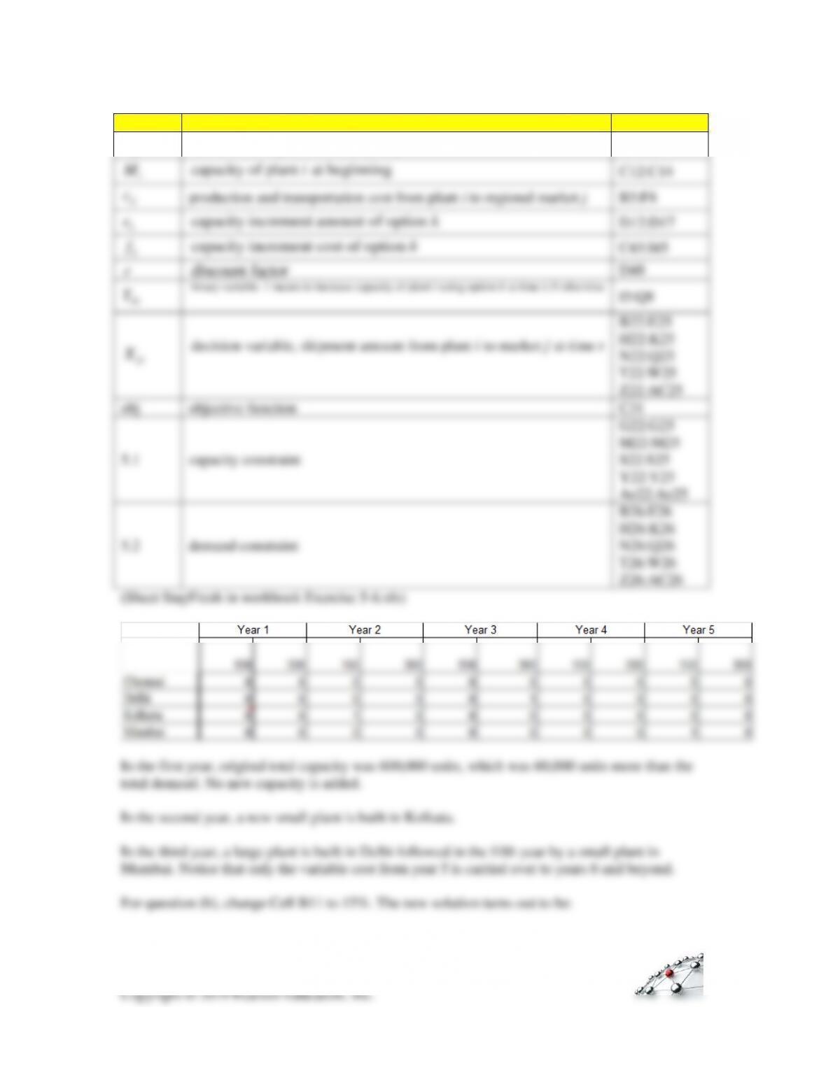
(Sheet StayFresh in workbook Exercise 5-6.xls)
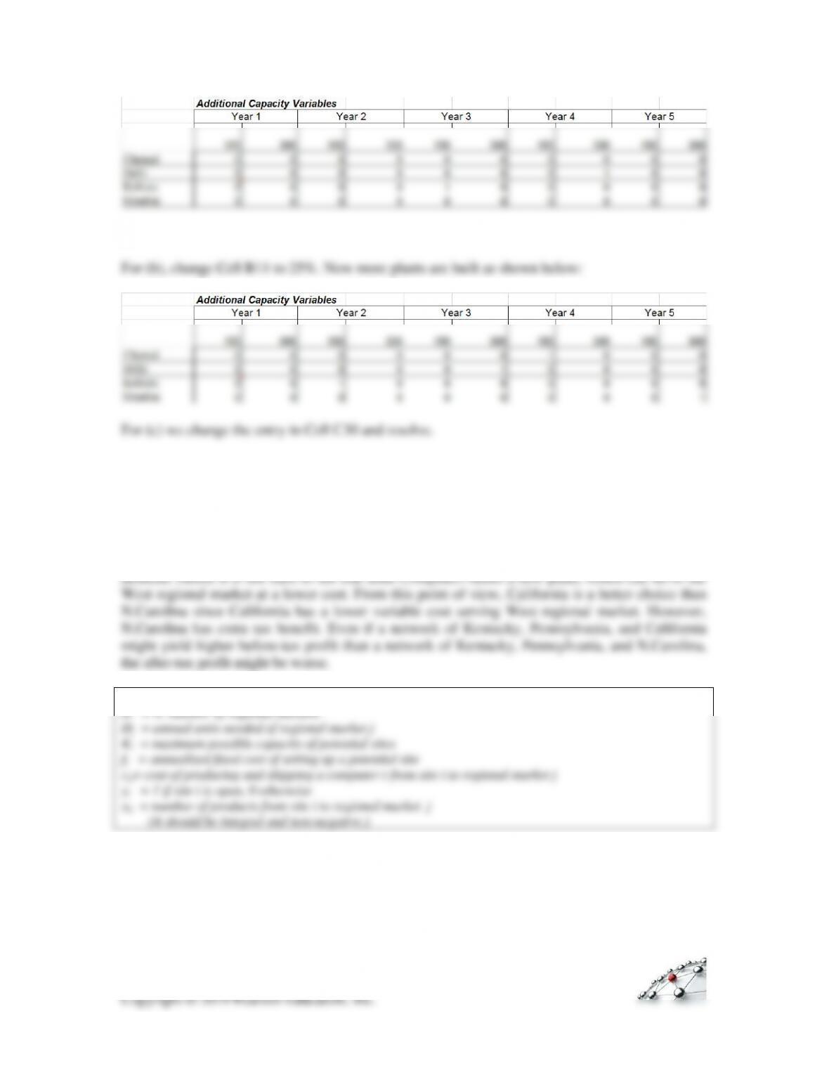
Given the lower growth rate, we build fewer plants.
7
(a)
Blue Computers has two plants in Kentucky and Pennsylvania, however, both have high variable
costs to serve the West regional market. On the other hand, West regional market has 2nd highest
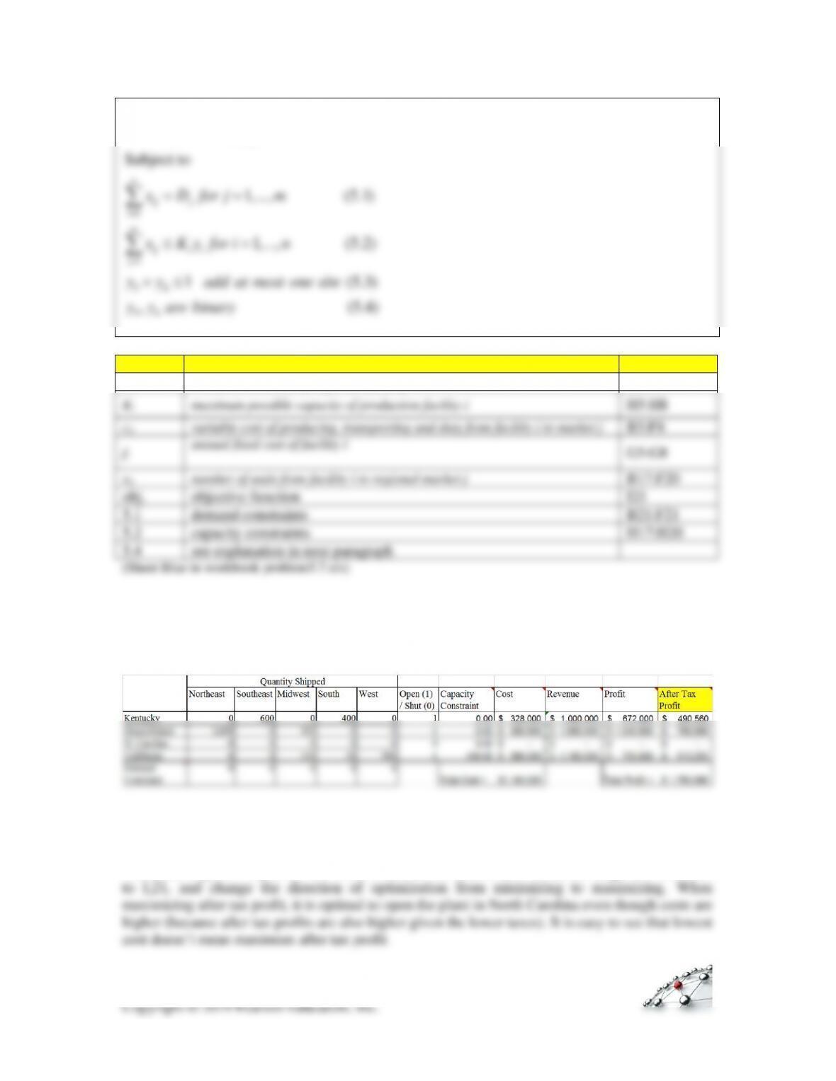
n = 2 potential sites
m = 4: number of regional markets
Dj = annual units needed of regional market j
Ki = maximum possible capacity of potential sites
fi = annualized fixed cost of setting up a potential site
cij= cost of producing and shipping a computer r from site i to regional market j
yi = 1 if site i is open, 0 otherwise
xij = number of products from site i to regional market j
(It should be integral and non-negative.)
1 1 1
1
1
34
34
Subject to
1,…, (5.1)
1,…, (5.2)
1 (5.3)
,
n n m
i i ij ij
i i j
n
ij j
i
m
ij i i
j
Min f y c x
x D for j m
x K y for i n
y y add at most one site
y y are binary
= = =
=
=
+
==
=
+
(5.4)
SYMBOL
INPUT
CELL
Dj
annual market size of regional market j
B9:F9
Ki
maximum possible capacity of production facility i
H5:H8
cij
variable cost of producing, transporting and duty from facility i to market j
B5:F8
fi
annual fixed cost of facility i
G5:G8
xij
number of units from facility i to regional market j
B17:F20
obj.
objective function
I21
5.1
demand constraints
B21:F21
5.2
capacity constraints
H17:H20
5.4
see explanation in next paragraph
When minimizing cost, it is optimal to open a plant in California as shown below (see worksheet
Lowest Cost).
(b)
We only need to change the objective function from minimize cost to maximize profit (see
worksheet Highest Profit). On the Excel sheet, all we need to do is to set the target cell from I21
Optimization model for Hot&Cold:
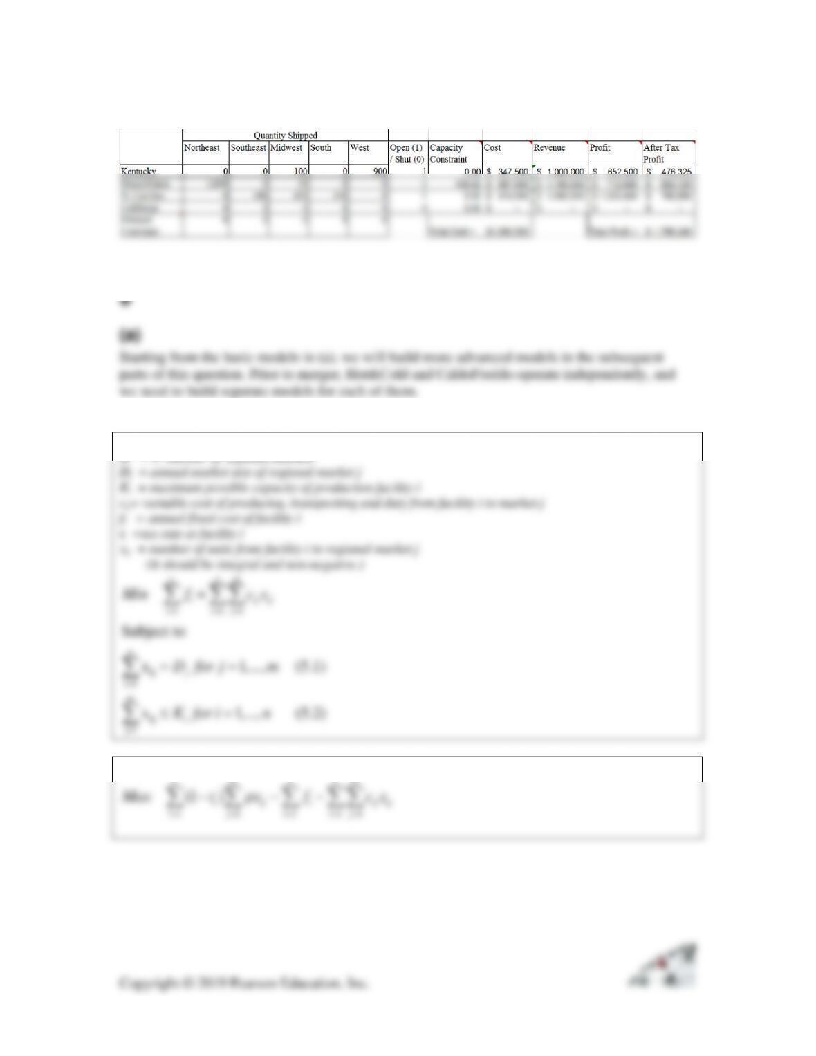
n = 3: Hot&Cold production facilities
m = 4: number of regional markets
Dj = annual market size of regional market j
Ki = maximum possible capacity of production facility i
cij= variable cost of producing, transporting and duty from facility i to market j
fi = annual fixed cost of facility i
ti =tax rate at facility i
xij = number of units from facility i to regional market j
(It should be integral and non-negative.)
1 1 1
n
ij
i1
m
ij
j1
Subject to
x 1 (5.1)
x 1 (5.2)
n n m
i ij ij
i i j
j
i
Min f c x
D for j ,…,m
K for i ,…,n
= = =
=
=
+
==
=
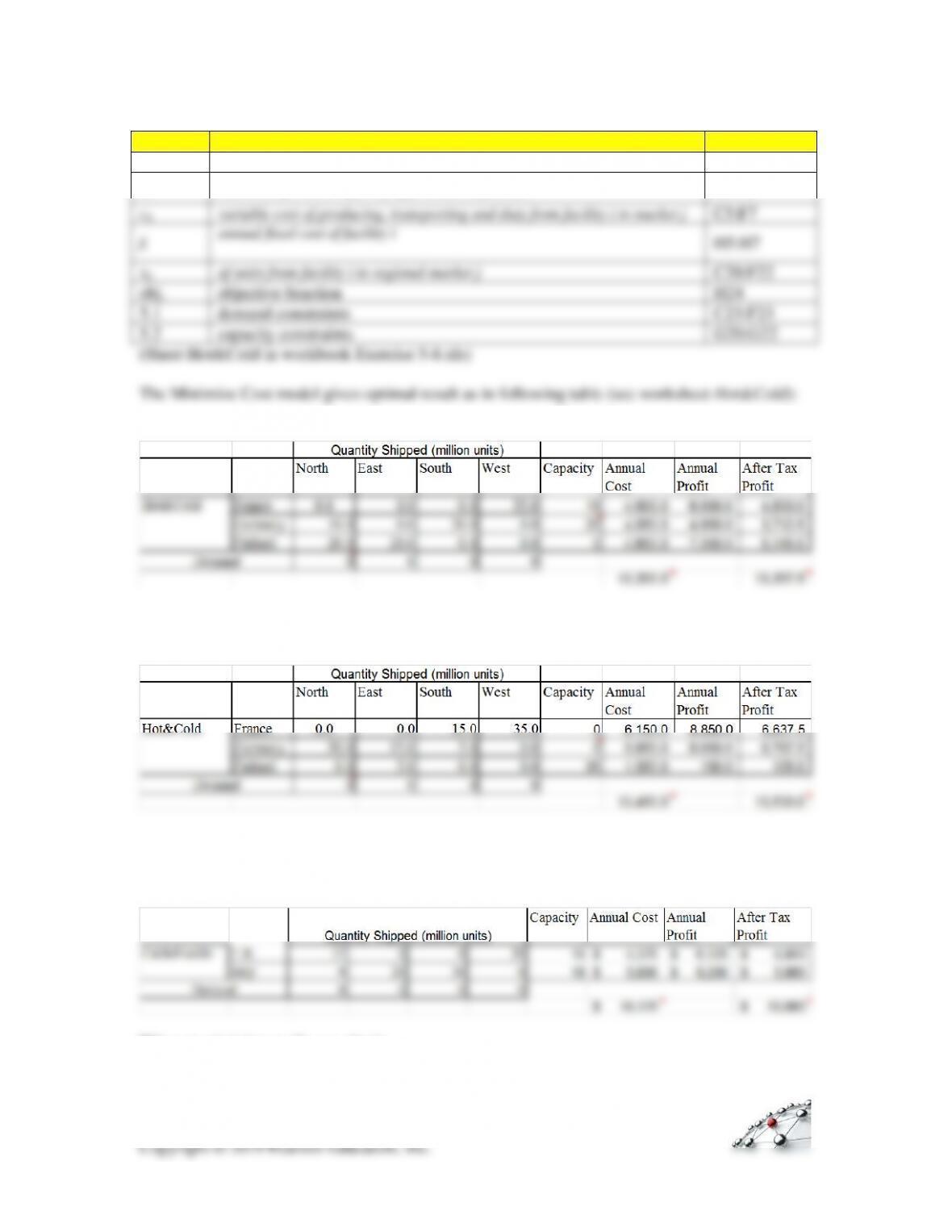
And replace above objective function to the following one to maximize after tax profit:
20
SYMBOL
INPUT
CELL
Dj
annual market size of regional market j
C8:F8
Ki
maximum possible capacity of production facility i
G5:G7
cij
variable cost of producing, transporting and duty from facility i to market j
C5:F7
fi
annual fixed cost of facility i
H5:H7
xij
of units from facility i to regional market j
C20:F22
obj.
objective function
H24
5.1
demand constraints
C23:F23
5.2
capacity constraints
G20:G22
The Maximize Profit model (change objective function to Max Cell J24) gives optimal result as
in following table (see worksheet Hot&Cold):
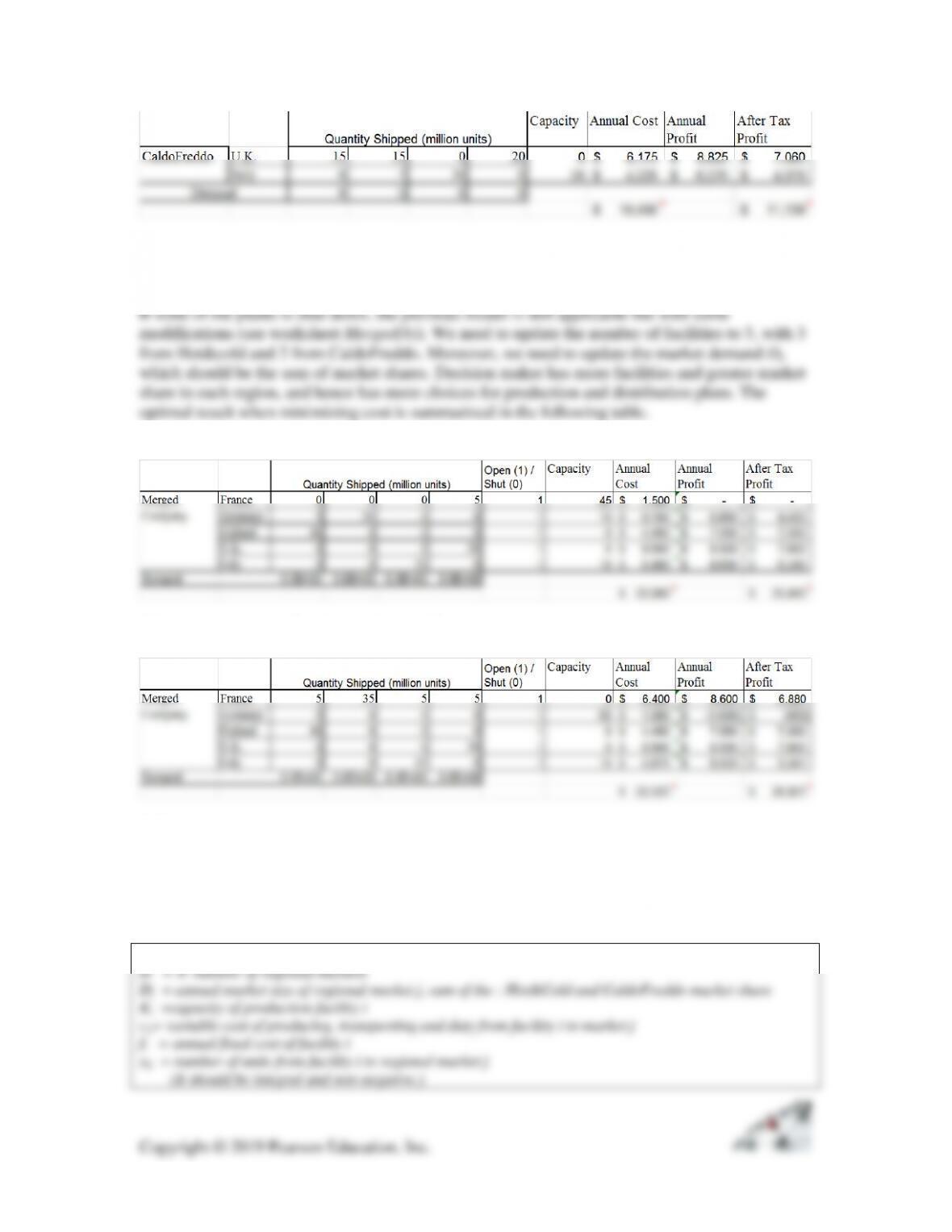
Moreover, we use the same model but with data from CaldoFreddo to get following optimal
production and distribution plan for CaldoFreddo (see worksheet CaldoFreddo):
When maximizing profits we obtain:
21
(b)
When maximizing profits the result is as follows:
(c)
This model is more advanced since it allows facilities to be shutdown. Accordingly we need more
variables to reflect this new complexity.
Optimization model for Sleekfon:
n = 5: Hot&Cold and CaldoFreddo production facilities
m = 4: number of regional markets
Dj = annual market size of regional market j, sum of the : Hot&Cold and CaldoFreddo market share
Ki =capacity of production facility i
cij= variable cost of producing, transporting and duty from facility i to market j
fi = annual fixed cost of facility i
xij = number of units from facility i to regional market j
(It should be integral and non-negative.)
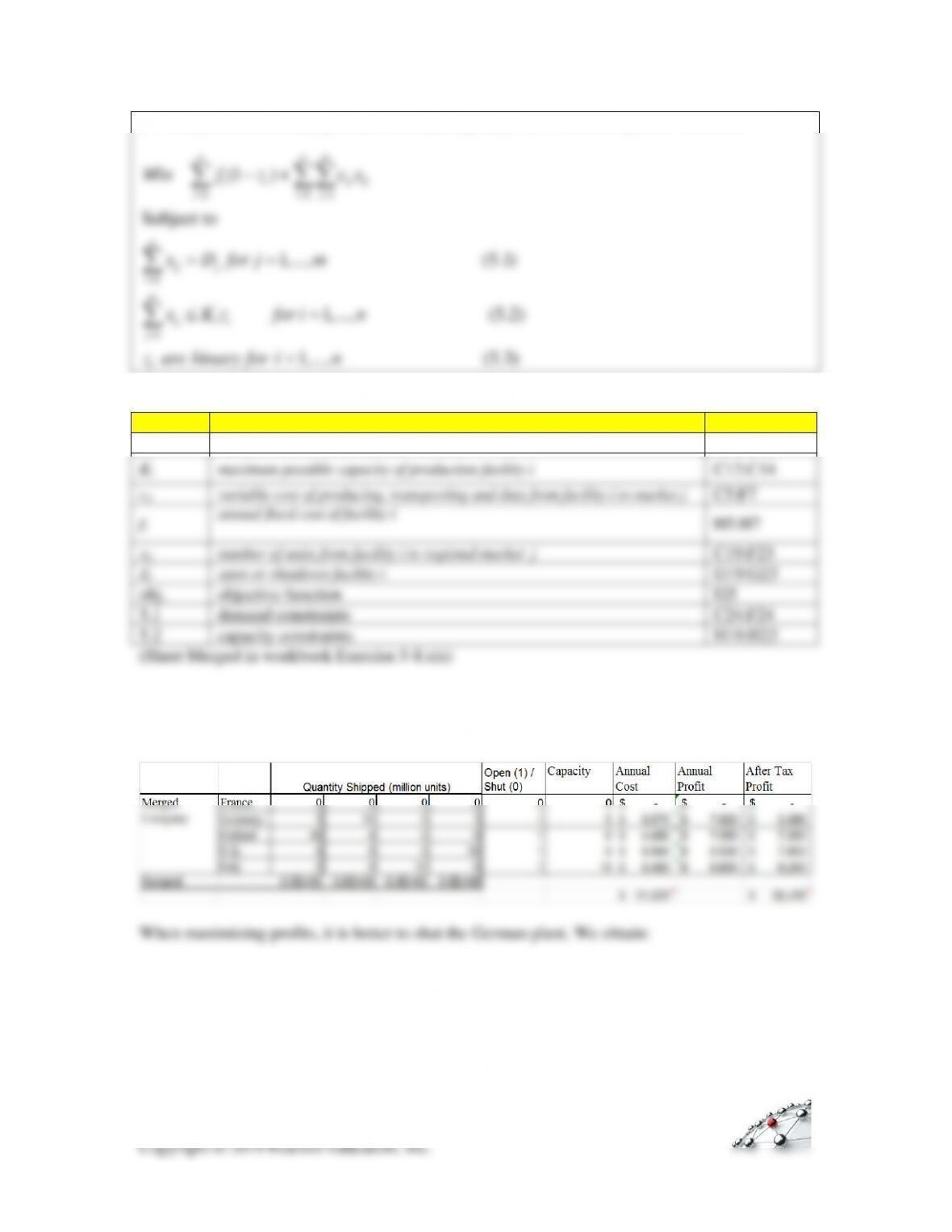
zi = binary variable indicating whether to shutdown facility i. zi =1 means to open it, 0 otherwise
1 1 1
1
1
(1 )
Subject to
1,…, (5.1)
1,…, (5.2)
1,…,
n n m
i i ij ij
i i j
n
ij j
i
m
ij i i
j
i
Min f z c x
x D for j m
x K z for i n
z are binary for i n
= = =
=
=
−+
==
=
=
(5.3)
SYMBOL
INPUT
CELL
Dj
annual market size of regional market j
C8:F8
Ki
maximum possible capacity of production facility i
C12:C14
cij
variable cost of producing, transporting and duty from facility i to market j
C5:F7
fi
annual fixed cost of facility i
H5:H7
xij
number of units from facility i to regional market j
C19:F23
Zi
open or shutdown facility i
G19:G23
obj.
objective function
I25
5.1
demand constraints
C24:F24
5.2
capacity constraints
H19:H23
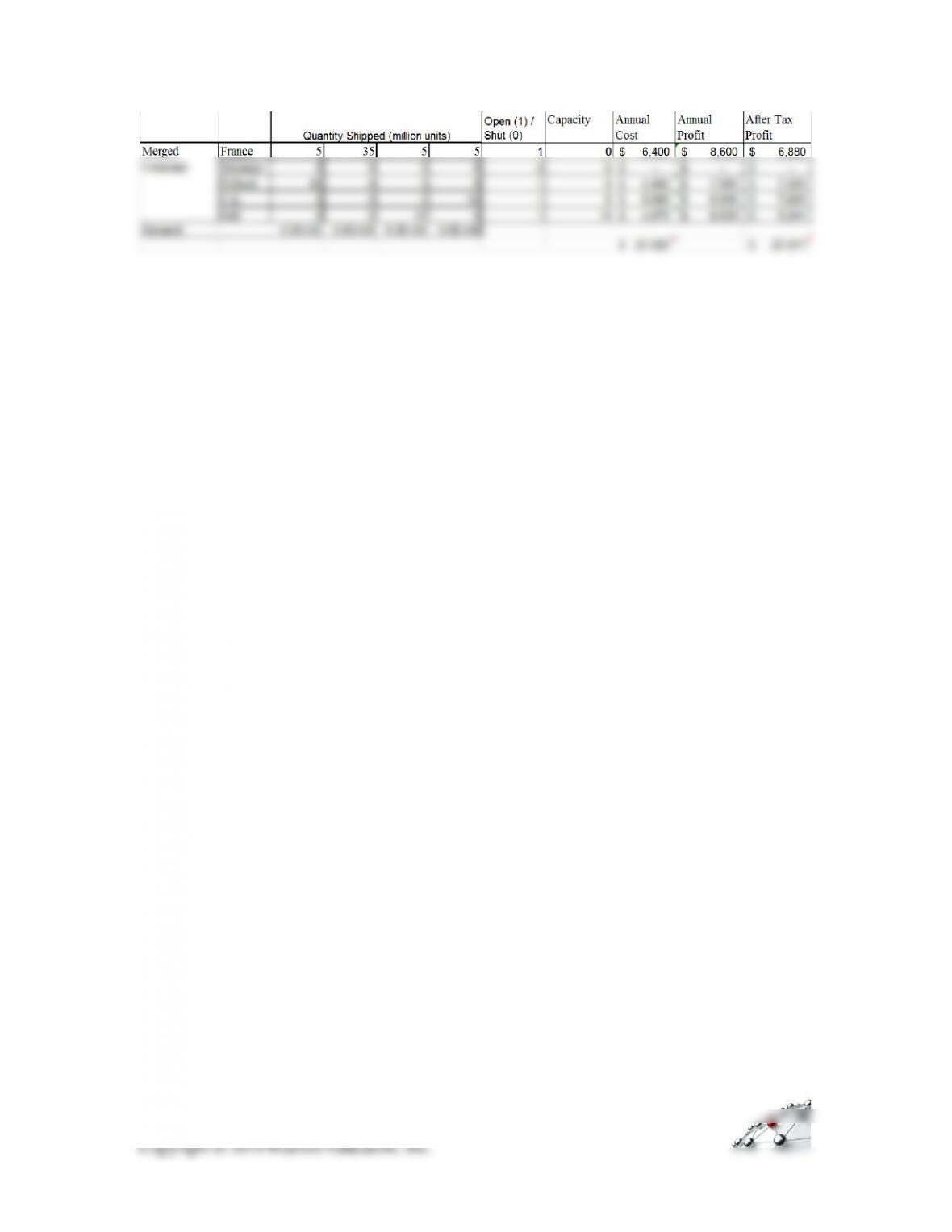
When minimizing cost, it is now optimal to close the French plant to achieve best objective value.
Following table shows the optimal configuration.
23