1
Chapter 5: Network Design in the Supply Chain
Exercise Solutions
1.
(a)
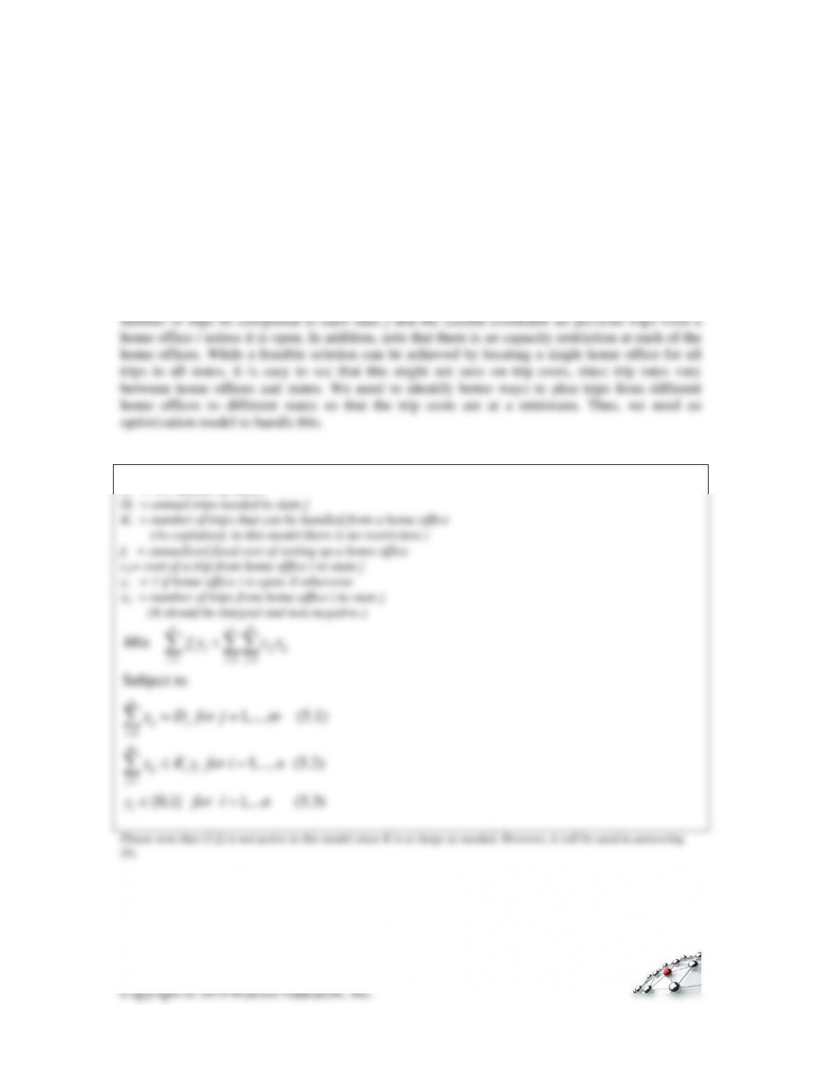
The objective of this model is to decide optimal locations of home offices, and number of trips
from each home office, so as to minimize the overall network cost. The overall network cost is a
combination of fixed costs of setting up home offices and the total trip costs.
There are two constraint sets in the model. The first constraint set requires that a specified
Optimization model:
n = 4: possible home office locations.
m = 16: number of states.
Dj = annual trips needed to state j
Ki = number of trips that can be handled from a home office
(As explained, in this model there is no restriction.)
fi = annualized fixed cost of setting up a home office
cij= cost of a trip from home office i to state j
yi = 1 if home office i is open, 0 otherwise
xij = number of trips from home office i to state j
(It should be integral and non-negative.)
1 1 1
n
i1
Subject to
1 (5.1)
n n m
i i ij ij
i i j
ij j
Min f y c x
x D for j ,…,m
= = =
=
+
==
2
SYMBOL
INPUT
CELL
Dj
annual trips needed to state j
E7:E22
cij
transportation cost from office i to state j
G7:G22,I7:I22,
K7:K22,M7:M22
fi
fixed cost of setting up office i
G26,I26,K26,M26
xij
number of consultants from office i to state j.
F7:F22,H7:H22,
J7:J22,L7:L22
obj.
objective function
M31
5.1
demand constraints
N7:N22
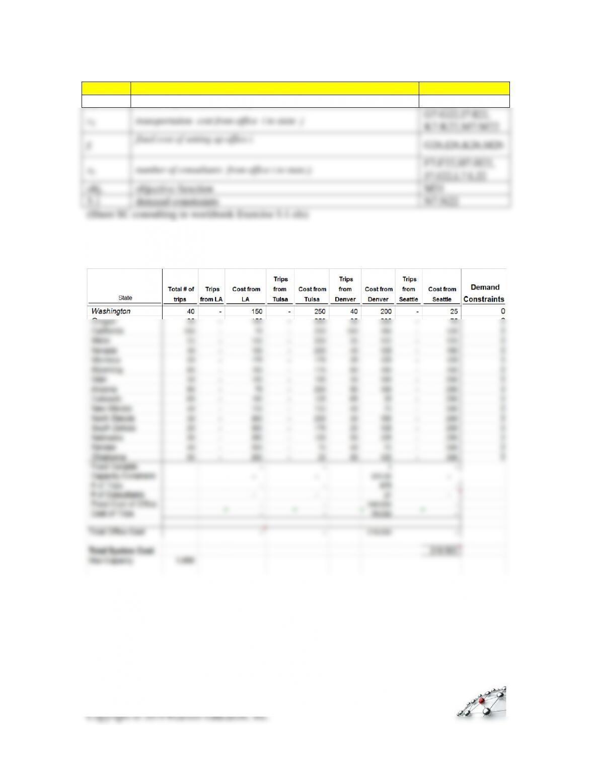
With this we solve the model to obtain the following results (see worksheet SC_Consulting (a)):
The number of consultants is calculated based on the constraint of 25 trips per consultant.
(b)
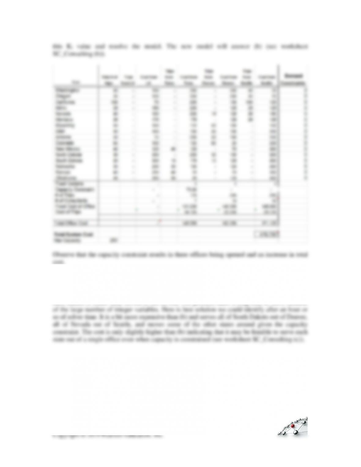
If at most 10 consultants are allowed at each home office, then we need to add one more
constraint that is, the total number of trips from an office may not exceed 250. Or in terms of the
optimization model, Ki, for all i, should have a value of 250. We can revise constraint (5.2) with
3
(c)
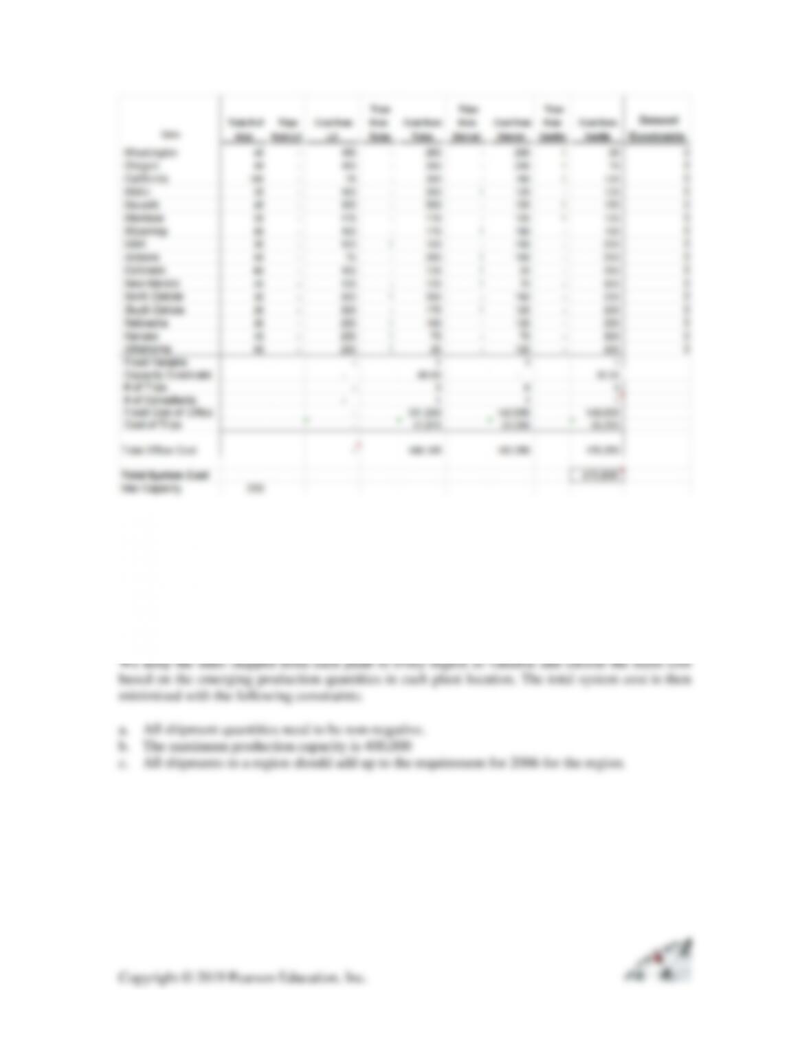
In this case, we need to restrict the markets served by each location to be 0/1 variables because
each market is either fully served or not served. The problem takes a long time to solve because
4
2.
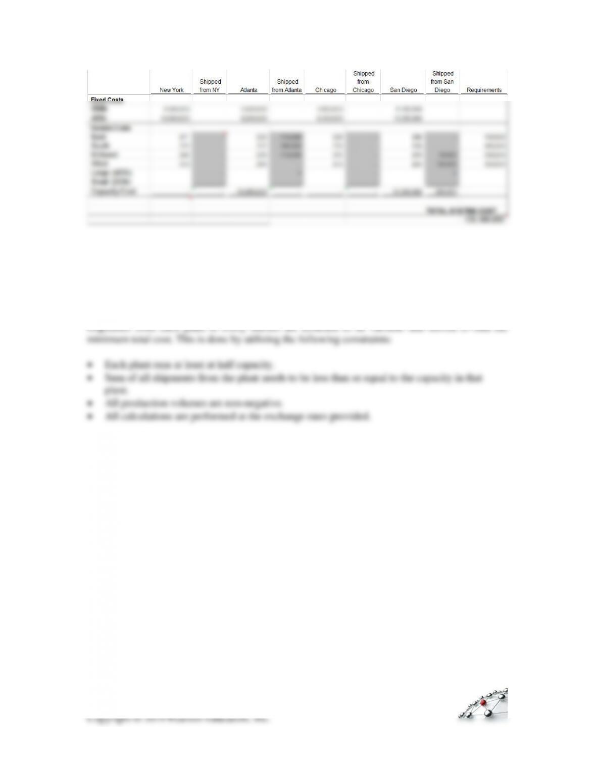
DryIce Inc. faces the trade-off between fixed cost (i.e., lower per item in a larger plant) versus the
cost of shipping and manufacturing. The typical scenarios that need to be considered are either
having regional manufacturing if the shipping costs are significant or have a centralized facility if
the fixed costs show significant economies to scale.
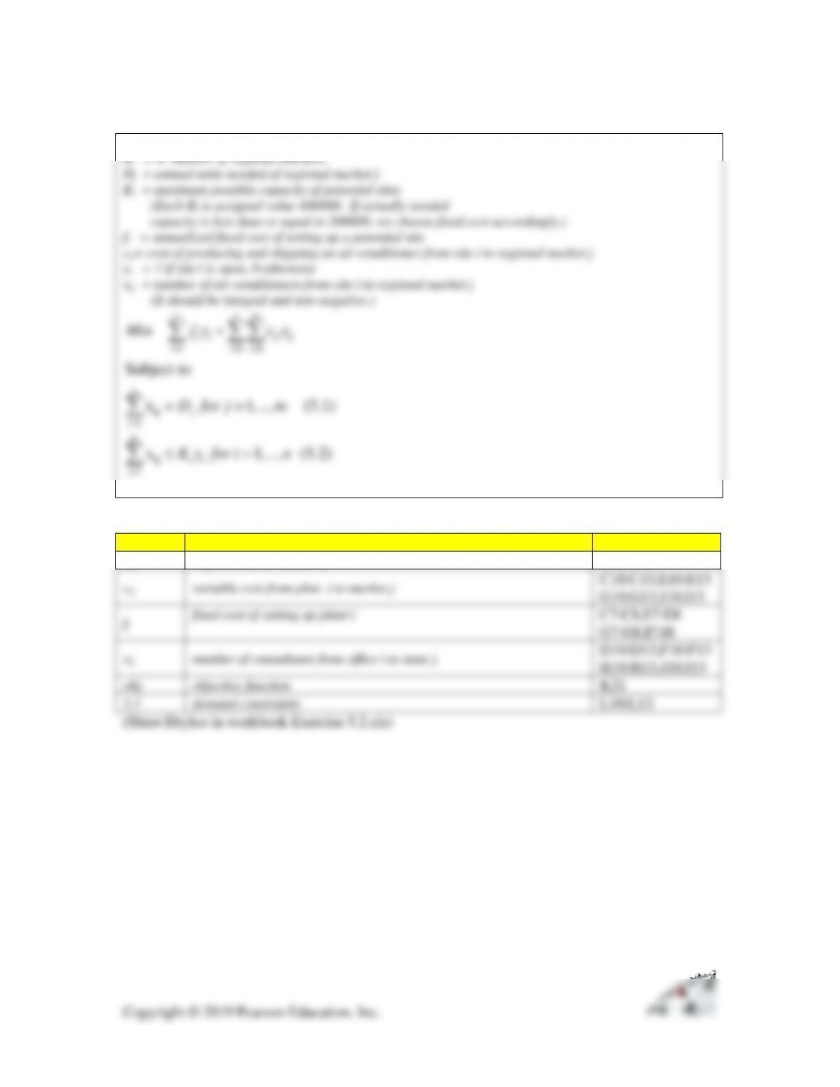
Optimization model:
n = 4: potential sites.
m = 4: number of regional markets.
Dj = annual units needed of regional market j
Ki = maximum possible capacity of potential sites
(Each Ki is assigned value 400000. If actually needed
capacity is less than or equal to 200000, we choose fixed cost accordingly.)
fi = annualized fixed cost of setting up a potential site
cij= cost of producing and shipping an air conditioner from site i to regional market j
yi = 1 if site i is open, 0 otherwise
xij = number of air conditioners from site i to regional market j
(It should be integral and non-negative.)
1 1 1
n
ij
i1
m
ij
j1
Subject to
x 1 (5.1)
x 1 (5.2)
n n m
i i ij ij
i i j
j
ii
Min f y c x
D for j ,…,m
K y for i ,…,n
= = =
=
=
+
==
=
SYMBOL
INPUT
CELL
Dj
requirement at market j
K10:K13
cij
variable cost from plan i to market j
C10:C13,E10:E13
G10:G13,I10:I13
fi
fixed cost of setting up plant i
C7:C8,E7:E8
G7:G8,I7:I8
xij
number of consultants from office i to state j.
D10:D13,F10:F13
H10:H13,J10:J13
obj.
objective function
K21
5.1
demand constraints
L10:L13
6
3
(a)
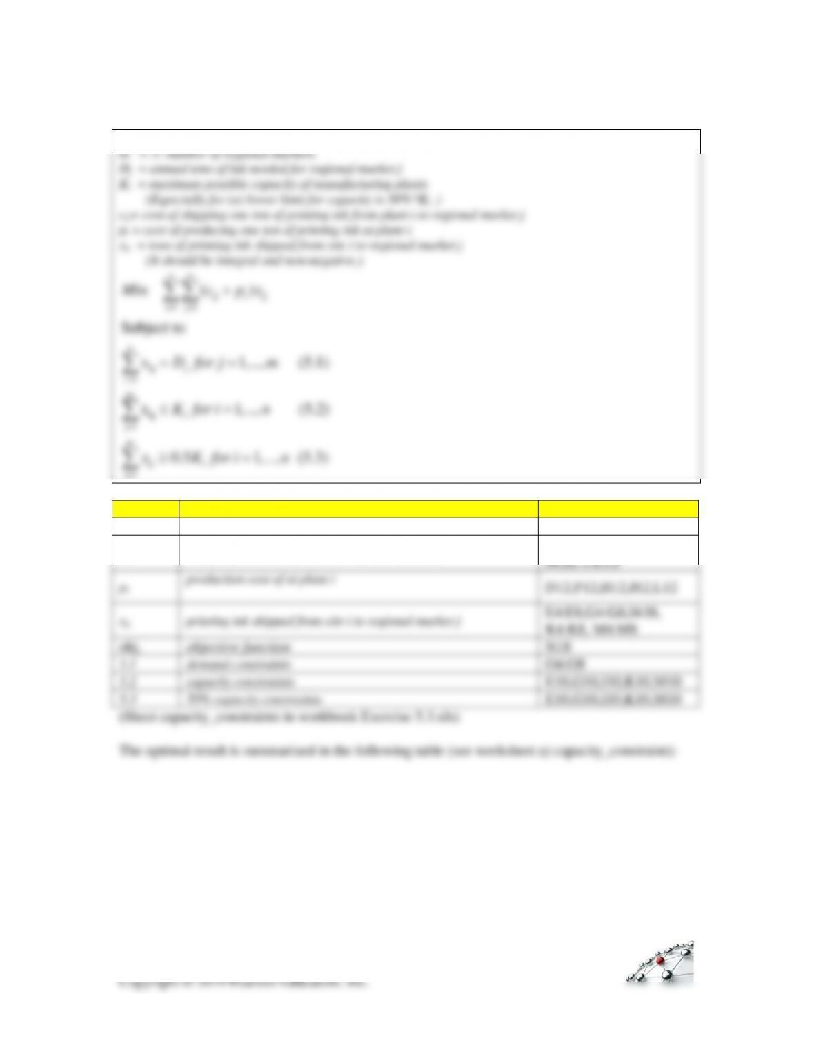
Sunchem can use the projections to build an optimization model as shown below. In this case, the
7
Optimization model:
n = 5: five manufacturing plants
m = 5: number of regional markets.
Dj = annual tons of ink needed for regional market j
Ki = maximum possible capacity of manufacturing plants
(Especially for (a) lower limit for capacity is 50%*Ki .)
cij= cost of shipping one ton of printing ink from plant i to regional market j
pi = cost of producing one ton of printing ink at plant i
xij = tons of printing ink shipped from site i to regional market j
(It should be integral and non-negative.)
11
n
ij
i1
m
ij
j1
m
j1
()
Subject to
x 1 (5.1)
x 1 (5.2)
0.5 1 (5.3)
nm
ij i ij
ij
j
i
ij i
Min c p x
D for j ,…,m
K for i ,…,n
x K for i ,…,n
==
=
=
=
+
==
=
=
SYMBOL
INPUT
CELL
Dj
annual demand at market j
N4:N8
cij
shipping cost from plant i to regional market j
D4:D8,F4:F8,H4:H8,
J4:J8, L4:L8
pi
production cost of at plant i
D12,F12,H12,J12,L12
xij
printing ink shipped from site i to regional market j
E4:E8,G4:G8,I4:I8,
K4:K8, M4:M8
obj.
objective function
N18
5.1
demand constraints
O4:O8
5.2
capacity constraints
E10,G10,I10,K10,M10
5.3
50% capacity constraints
E10,G10,I10,K10,M10
8
(b)
(c)
9
(d)
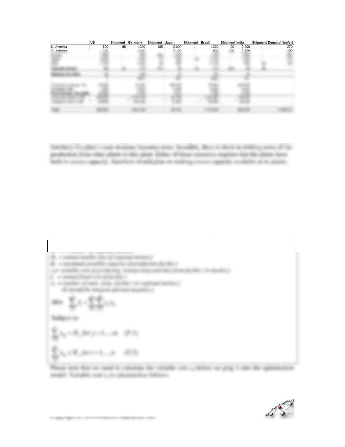
It is clear that fluctuations in exchange rates will change the cost structure of each plant. If the
cost at a plant becomes too high, there is merit in shifting some of the production to another plant.
4
(a)
Starting from the basic models in (a), we will build more advanced models in the subsequent
parts of this question. Prior to merger, Sleekfon and Sturdyfon operate independently, and so we
need to build separate models for each of them.
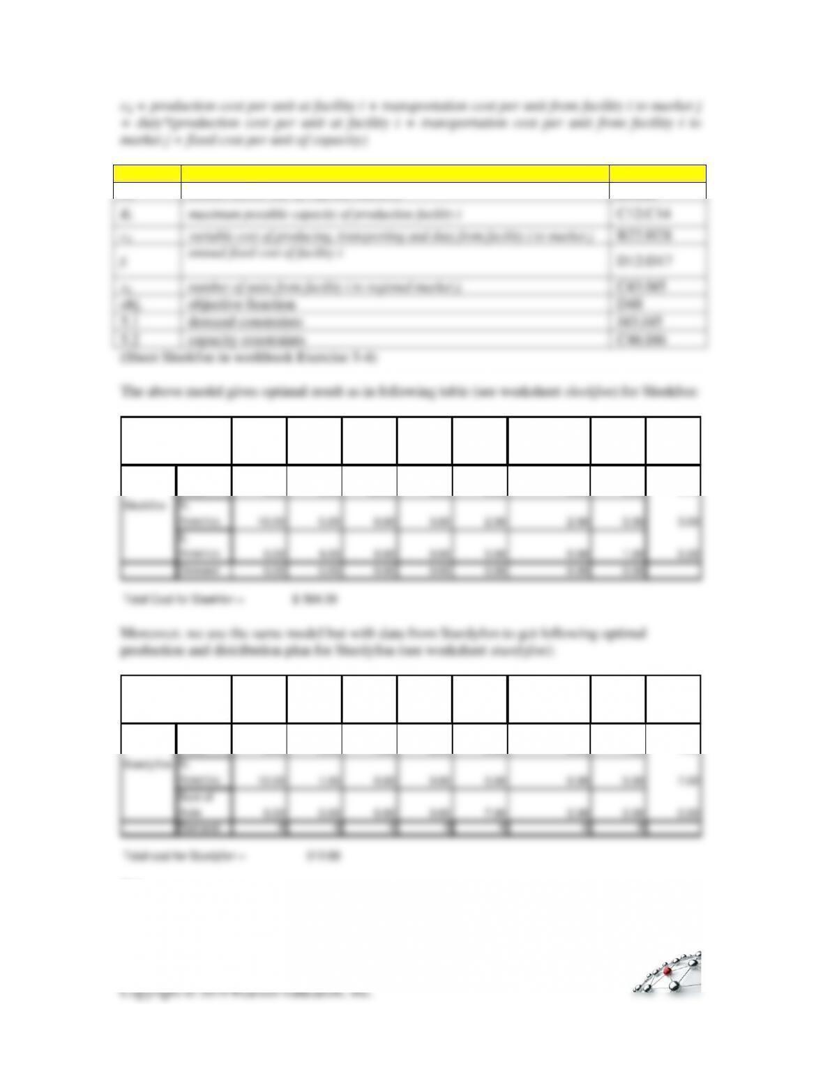
Optimization model for Sleekfon:
n = 3: Sleekfon production facilities.
m = 7: number of regional markets.
Dj = annual market size of regional market j
Ki = maximum possible capacity of production facility i
cij= variable cost of producing, transporting and duty from facility i to market j
fi = annual fixed cost of facility i
xij = number of units from facility i to regional market j
(It should be integral and non-negative.)
1 1 1
n
Subject to
n n m
i ij ij
i i j
Min f c x
= = =
+
10
SYMBOL
INPUT
CELL
Dj
annual market size of regional market j
B4:H4
Ki
maximum possible capacity of production facility i
C12:C14
cij
variable cost of producing, transporting and duty from facility i to market j
B22:H28
fi
annual fixed cost of facility i
D12:D17
xij
number of units from facility i to regional market j.
C43:I45
obj.
objective function
D48
5.1
demand constraints
J43:J45
5.2
capacity constraints
C46:I46
N.
America
S.
America
Europe
(EU)
Europe
(Non EU)
Japan
Rest of
Asia/Australia
Africa Capacity
Europe
(EU)
0.00 0.00 20.00 0.00 0.00 0.00 0.00 0.00
Sleekfon
N.
America
10.00 0.00 0.00 3.00 2.00 2.00 0.00 3.00
S.
America
0.00 4.00 0.00 0.00 0.00 0.00 1.00 5.00
Demand 0.00 0.00 0.00 0.00 0.00 0.00 0.00
Total Cost for Sleekfon = 564.39$
Quantity Shipped
N.
America
S.
America
Europe
(EU)
Europe
(Non EU)
Japan
Rest of
Asia/Australia
Africa Capacity
Europe
(EU)
0.00 0.00 4.00 8.00 0.00 0.00 1.00 7.00
Sturdyfon
N.
America
12.00 1.00 0.00 0.00 0.00 0.00 0.00 7.00
Rest of
Asia
0.00 0.00 0.00 0.00 7.00 3.00 0.00 0.00
Demand 0 0 0 0 0 0 0
Total cost for Sturdyfon = 512.68
Quantity Shipped
(b)
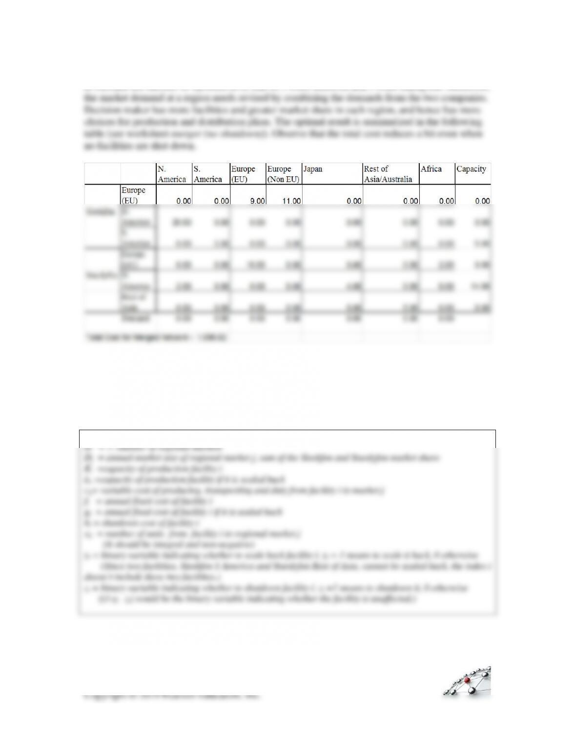
Under conditions of no plant shutdowns, the previous model is still applicable. However, we need
to increase the number of facilities to 6, that is, 3 from Sleekfon and 3 from Sturdyfon. Moreover,
(c)
This model is more advanced since it allows facilities to be scaled down or shutdown.
Accordingly, we need more variables to reflect this new complexity.
Optimization model for Sleekfon:
n = 6: Sleekfon and Sturdyfon production facilities
m = 7: number of regional markets
Dj = annual market size of regional market j, sum of the Sleekfon and Sturdyfon market share
Ki =capacity of production facility i
Li =capacity of production facility if it is scaled back
cij= variable cost of producing, transporting and duty from facility i to market j
fi = annual fixed cost of facility i
gi = annual fixed cost of facility i if it is scaled back
hi = shutdown cost of facility i
xij = number of units from facility i to regional market j
(It should be integral and non-negative)
yi = binary variable indicating whether to scale back facility i. yi = 1 means to scale it back, 0 otherwise
(Since two facilities, Sleekfon S America and Sturdyfon Rest of Asia, cannot be scaled back, the index i