Example 16-1 Pricing to Multiple Segments
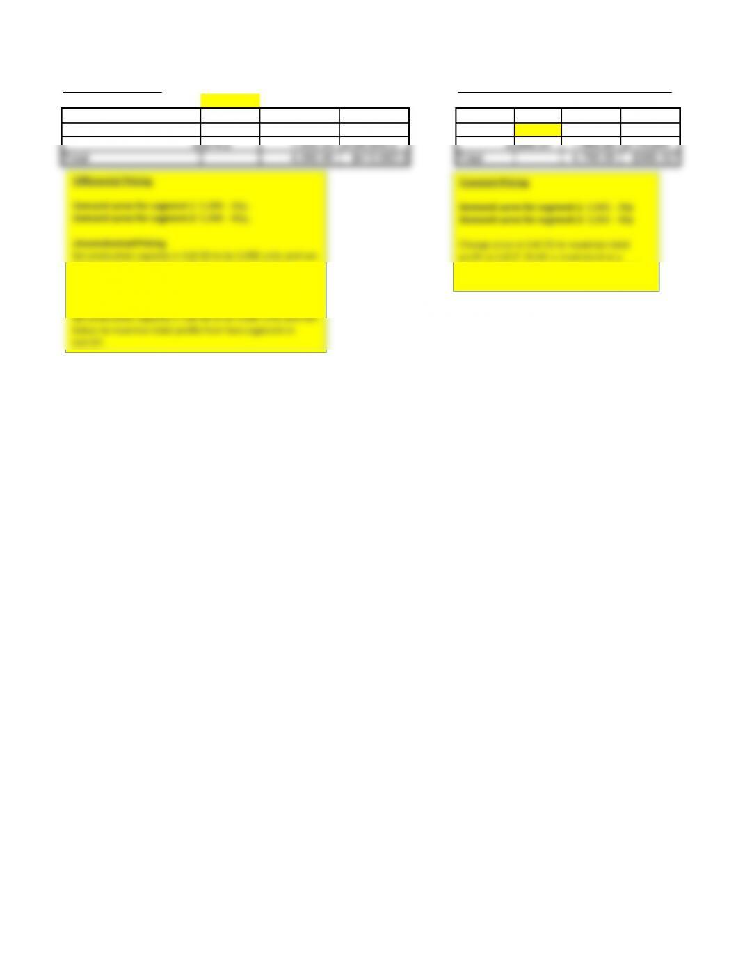
Differential Pricing Constant Pricing w/o capacity constraint
Production Capacity = 4,000
Segment Price Demand Profit Segment Price Demand Profit
1 $141.7 2,166.67 $285,277.8 1 $88.33 3,233.40 $253,272
2 $79.2 1,833.33 $126,805.6 2 $88.33 1,466.80 $114,894
Total 4,000.00 $412,083.3 Total 4,700.20 $368,167
Differential Pricing
Demand curve for segment 1: 5,000 – 20p1
Demand curve for segment 2: 5,000 – 40p2
Unconstrained Pricing
Set production capacity in Cell B3 to be 5,000 units and run
Solver to maximize total profits from two segments in
Cell D7.
Constrained Pricing
Set production capacity in Cell B3 to be 4,000 units and run
Solver to maximize total profits from two segments in
Cell D7.
Constant Pricing
Demand curve for segment 1: 5,000 – 20p
Demand curve for segment 2: 5,000 – 40p
Change price in Cell G5 to maximize total
profit in Cell I7. Profit is maximized at a
price of 88.33 without a capacity constraint.
Example 16-2 Allocating Capacity to Uncertain Demand from Multiple Segments
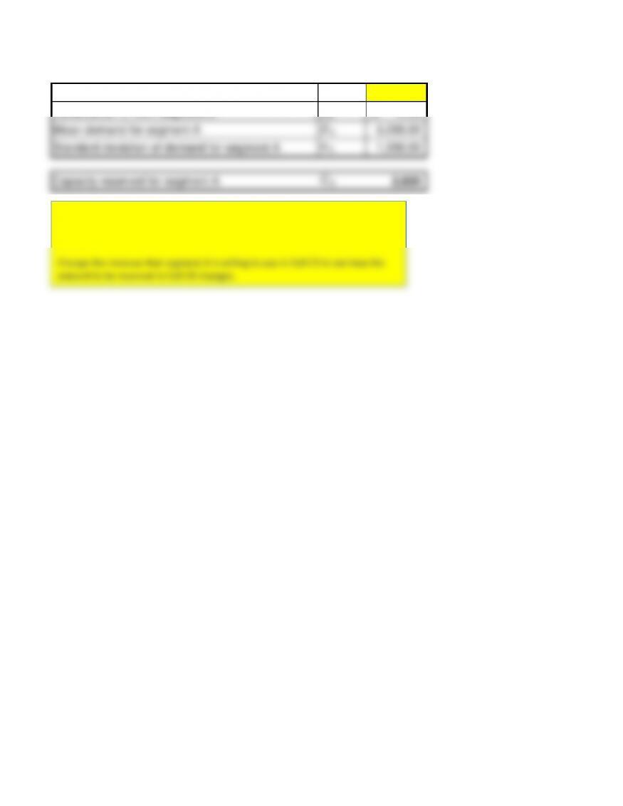
Revenue/cu. ft. from Segment A
pA3.50$
Revenue/cu. ft. from Segment B
pB2.00$
Mean demand for segment A
DA3,000.00
Standard deviation of demand for segment A
σA1,000.00
Capacity reserved for segment A
CA2,820
Initially set the revenue from the high-priced segment (A) in Cell C3 to $3.50.
The capacity to be reserved for the higher-priced segment A is calculated in
Cell C8.
Change the revenue that segment A is willing to pay in Cell C3 to see how the
amount to be reserved in Cell C8 changes.
Example 16-3 Dynamic Pricing
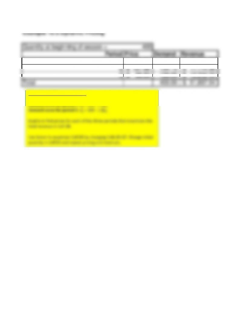
Quantity at beginning of season = 400
Period Price Demand Revenue
1 162.20$ 137.80 22,351.28$
2 127.58$ 134.15 17,114.36$
3 95.53$ 128.05 12,232.30$
Total 400.00 51,697.94$
Example 16-3 (Dynamic Pricing)
Demand curve for period 1: d1= 300 – p1
Demand curve for period 2: d2= 300 – 1.3p2
Demand curve for period 3: d3= 300 – 1.8p3
Goal is to find prices for each of the three periods that maximizes the
total revenue in Cell D8.
Use Solver to maximize Cell D8 by changing Cells B5:B7. Change initial
quantity in Cell B3 and repeat pricing and revenues.
Example 16-3 (Fixed Pricing)
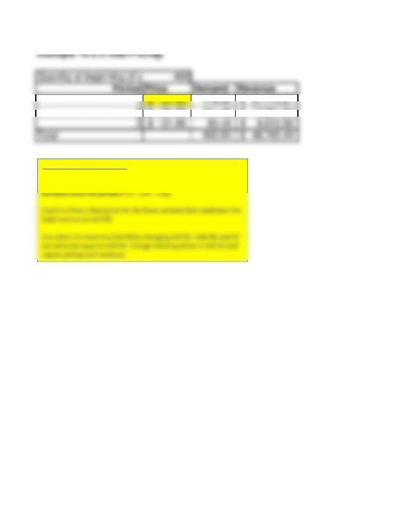
Quantity at beginning of season =
400
Period Price Demand Revenue
1 121.95$ 178.05 21,713.27$
2 121.95$ 141.46 17,251.64$
3 121.95$ 80.49 9,815.59$
Total 400.00 48,780.49$
Example 16-3 (Fixed Pricing)
Demand curve for period 1: d1= 300 – p1
Demand curve for period 2: d2= 300 – 1.3p2
Demand curve for period 3: d3= 300 – 1.8p3
Goal is to find a fixed price for the three periods that maximizes the
total revenue in Cell D8.
Use Solver to maximize Cell D8 by changing Cell B5. Cells B6 and B7
are set to be equal to Cell B5. Change initial quantity in Cell B3 and
repeat pricing and revenues.
Example 16-4 Evaluating Initial Quantity with Dynamic Pricing
Cost per unit = 100.00$
Quantity at beginning of season = 245
Period Price Demand Revenue
1 200.00$ 100 20,000.00$
2 165.38$ 85 14,057.70$
3 133.33$ 60 8,000.01$
Total 245 42,057.71$
Profit = 17,557.69$
Example 16-4 (Evaluating quantity with dynamic pricing))
Demand curve for period 1: d1= 300 – p1
Demand curve for period 2: d2= 300 – 1.3p2
Demand curve for period 3: d3= 300 – 1.8p3
Goal is to find an initial order quantity that maximizes season profits in Cell D9
given a unit cost in Cell B2.
Use Solver to maximize the profit in Cell D9 by changing Cells B3 (initial quantity)
and Cells B5:B7 (dynamic prices).
Example 16.4 (The challenge of strategic customers)
Cost per unit = 100.00$
Quantity at beginning of season = 245
Period
Price
without
strategic
customers
Demand
without
strategic
customers
Revenue
without
strategic
customers
Price with
strategic
customers
Demand
with
strategic
customers
Revenue with
strategic
customers
1 200.00$ 100 20,000.00$ 200.00$ 80 16,000.00$
2 165.38$ 85 14,057.30$ 165.38$ 50 8,269.00$
3 133.33$ 60 7,999.80$ 102.78$ 115 11,819.45$
Total 42,057.10$ 245 36,088.45$
Profit = 17,557.08$ Profit = 11,588.43$
Example 16-4 with strategic customers
We assume that the retailer starts the season with 245 units as in Example16-4. When customers are
not strategic and do not delay their demand, the monthly pricing is in cells B5:B7, monthly demand in
cells C5:C7. Total revenue in the absence of strategic customers is given in Cell D8.
Given that customers are strategic, some of the customers who would have bought in months 1 or 2
delay their purchase to month 3. The sales in months 1 and 2 with strategic customers are entered in
Cells F5 and F6. All left over inventory (245 – F5-F6) must be sold in month 3. The retailer thus
prices in month 3 (Cell B7) to sell all available quantity given the demand curve d3= 300 – 1.8p3. In other
words, p3(in Cell E7) = (300 – Leftover quantity)/1.8.
Total profit with strategic customers is shown in Cell G8. Change the amount sold in Cells F5 and F6 to
see how the profit in Cell G9 (with strategic customers) changes.
Example 16-4 (Fixed Pricing with strategic customers)
Unit cost = 100$
Quantity at beginning of season =
245
Period Price Demand Revenue
1 159.76$ 140.24 22,404.82$
2 159.76$ 92.32 14,748.22$
3 159.76$ 12.44 1,987.21$
Total 245.00 39,140.24$
Profit 14,640.24$
Example 16-4 (Fixed Pricing with strategic customers)
Demand curve for period 1: d1= 300 – p1
Demand curve for period 2: d2= 300 – 1.3p2
Demand curve for period 3: d3= 300 – 1.8p3
Goal is to find a fixed price for the three periods that maximizes the
total profit in Cell D9.
Use Solver to maximize Cell D9 by changing Cell B3 & B5. Cells B6 and B7
are set to be equal to Cell B5.
Example 16-5 Overbooking
Capacity available at apparel supplier 5,000
Cost per unit of wasted capacity, Cw10.00$
Cost per unit of capacity shortage, Cs5.00$
Probability that cancellations will be less than or equal to the
optimal booking level, s*
0.667
Cancellation distribution is fixed
Demand cancellation mean 800
Std deviation of demand cancellation 400
Optimal overbooking level, O*972
Optimal order level 5,972
Cancellation distribution is order size dependent
Average cancellation rate 15%
Coefficient of variation of cancellations 0.5
O evaluated using Equation 16.8 1,115
Overbooking level, O*1,115
Optimal order level 6,115
Cell B11 contains the optimal overbooking level
(obtained using Equation 16.7) assuming a fixed
cancellation distribution with mean
in Cell B9 and standard deviation in Cell B10.
To obtain the optimal overbooking level, change
Cell B18 until it equals the number in Cell B17.
When the two are equal, Cell B18 contains the
optimal overbooking level (solution to
Equation 16.8).
Example 16-6 Long-term Bulk Contracts versus the Spot Market
Mean transportation needs 10,000,000
Std dev 4,000,000
Bulk contract cost, cB10,000$
Spot market cost, cS12,500$
Optimal probability p* (Equation 16.9) 0.2
Optimal order amount Q* (Equation 16.10) 6,633,515