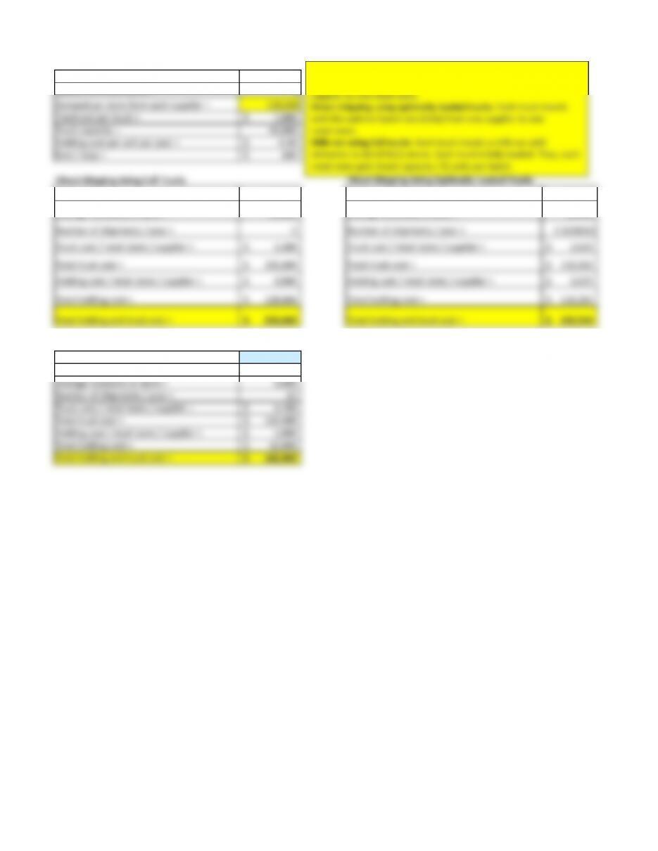
Input Data
Number of suppliers = 4
Number of retail stores = 8
Demand per store from each supplier = 120,000
Fixed cost per truck = 1,000$
Truck capacity = 40,000
Holding cost per unit per year = 0.20$
Cost / stop = 100$
Direct Shipping Using Full Trucks Direct Shipping Using Optimally Loaded Trucks
Batch size, Q = 40,000 Optimal batch size = 36,332
Average inventory at store = 20,000 Average inventory at store = 18,166
Number of shipments / year = 3 Number of shipments / year = 3.3028913
Truck cost / retail store / supplier = 3,300$ Truck cost / retail store / supplier = 3,633$
Total truck cost = 105,600$ Total truck cost = 116,262$
Holding cost / retail store / supplier = 4,000$ Holding cost / retail store / supplier = 3,633$
Total holding cost = 128,000$ Total holding cost = 116,262$
Total holding and truck cost = 233,600$ Total holding and truck cost = 232,524$
Milk Run Using Full Trucks
Number of stores / truck 4
Batch size = 10,000
Average inventory at store = 5,000
Number of shipments / year = 12
Truck cost / retail store / supplier = 4,200$
Total truck cost = 134,400$
Holding cost / retail store / supplier = 1,000$
Total holding cost = 32,000$
Total holding and truck cost = 166,400$
We present the following analysis:
Direct shipping using full trucks: Each truck travels full from one
supplier to one retail store.
Direct shipping using optimally loaded trucks: Each truck travels
with the optimal batch size (EOQ) from one supplier to one
retail store.
Milk run using full trucks: Each truck travels a milk run with
deliveries to k(Cell B21) stores. Each truck is fully loaded. Thus, each
retail store gets (truck capacity / k) units per batch.
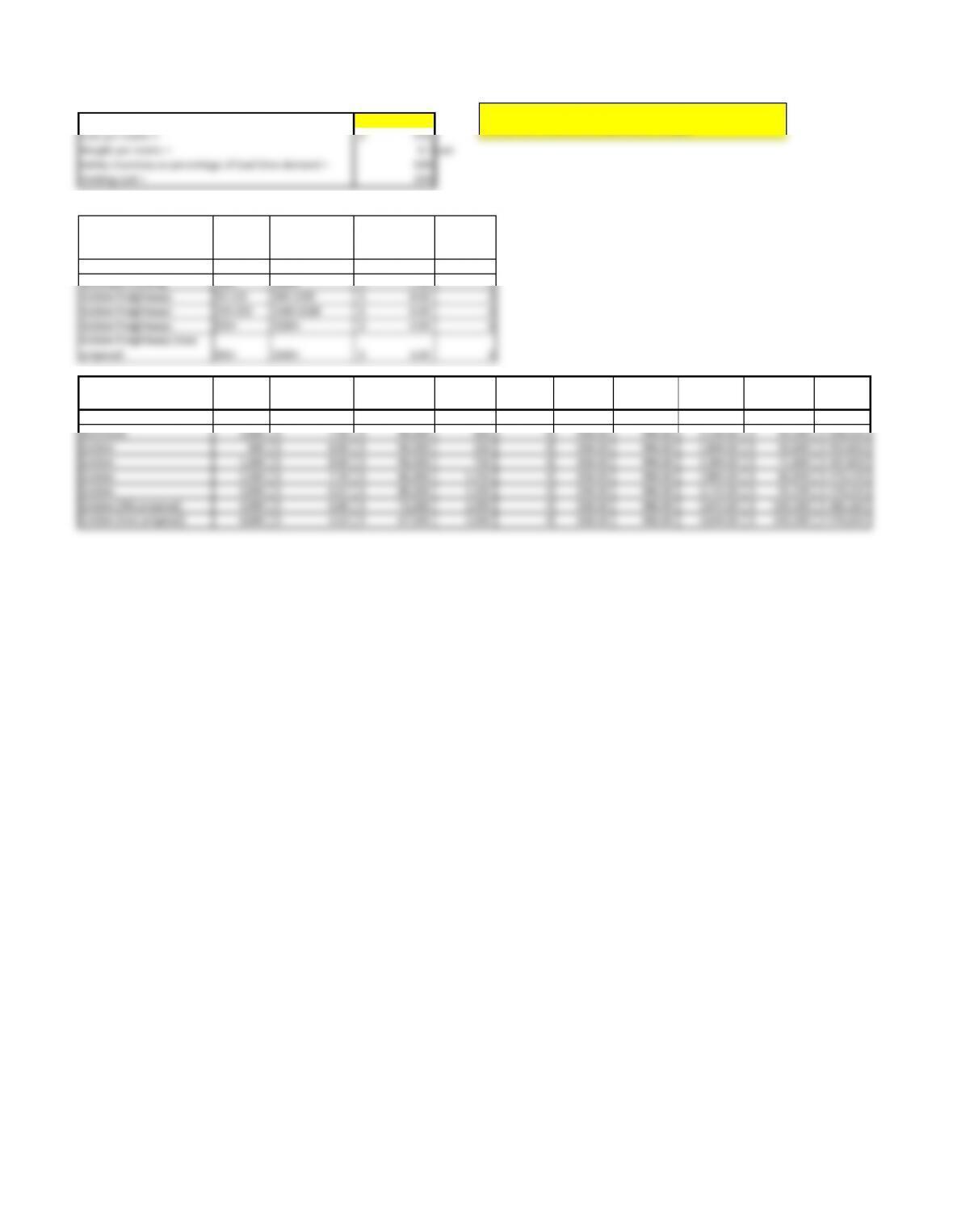
Example 14-2: Trade-offs when selecting transportation mode
Number of motors purchased per year = 120,000
Cost per motor = 120$
Weight per motor = 0.1 cwt
Safety inventory as percentage of lead time demand = 50%
Holding cost = 25%
Transportation proposals for Eastern Electric
Carrier
Quantity
shipped
(cwt)
Quantity shipped
(motors)
Shipping cost
($/cwt)
Transit time
(days)
AM Railroad 200+ 2000+ 6.50$ 5
Northeast trucking 100+ 1000+ 7.50$ 3
Golden Freightways 50-150 500-1500 8.00$ 3
Golden Freightways 150-250 1500-2500 6.00$ 3
Golden Freightways 250+ 2500+ 4.00$ 3
Golden Freightways (new
proposal)
250+ 2500+ 3.00$ 3
Transportation Alternative
Lot Size
(Motors)
Transportation
Cost/cwt
Transportation
Cost
Cycle
Inventory
Lead Time
(days)
Safety
Inventory
In-Transit
Inventory
Total
Inventory
Holding Cost Total Cost
AM Rail 2,000 6.50$ 78,000$ 1,000 6 986.00 1,644.00 3,630.00 108,900$ 186,900$
Northeast 1,000 7.50$ 90,000$ 500 4 658.00 986.00 2,144.00 64,320$ 154,320$
Golden 500 8.00$ 96,000$ 250 4 658.00 986.00 1,894.00 56,820$ 152,820$
Golden 1,500 8.00$ 96,000$ 750 4 658.00 986.00 2,394.00 71,820$ 167,820$
Golden 2,500 7.20$ 86,400$ 1,250 4 658.00 986.00 2,894.00 86,820$ 173,220$
Golden 3,000 6.67$ 80,000$ 1,500 4 658.00 986.00 3,144.00 94,320$ 174,320$
Golden (Old proposal) 4,000 6.00$ 72,000$ 2,000 4 658.00 986.00 3,644.00 109,320$ 181,320$
Golden (new proposal) 4,000 5.63$ 67,500$ 2,000 4 658.00 986.00 3,644.00 109,320$ 176,820$
Change the annual demand in Cell D3 in increments of 120,000
to see how the preferred alternative changes.
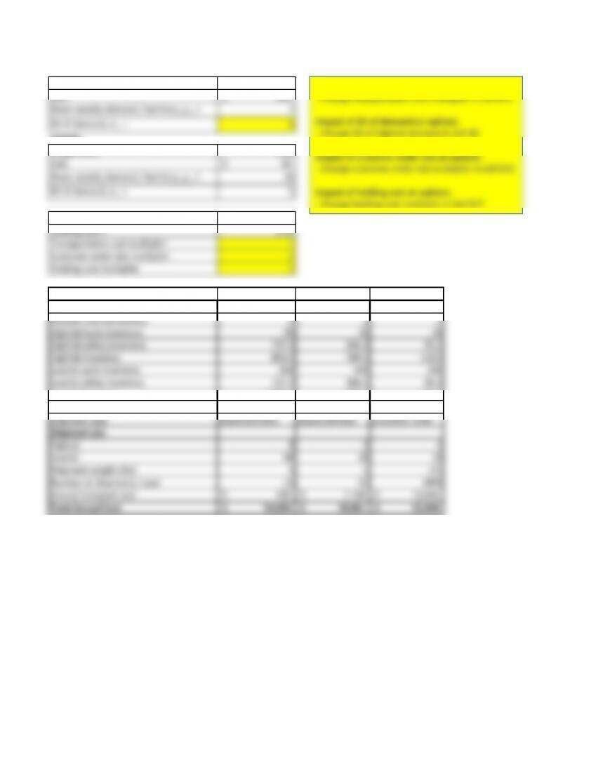
Example 14-3: Trade-offs When Aggregating Inventory
Highval
Weight (lbs) 0.1
Cost 200$
Mean weekly demand / territory, µH = 2
SD of demand, σH = 5
Lowval
Weight (lbs) 0.04
Cost 30$
Mean weekly demand / territory, µL = 20
SD of demand, σL = 5
Cycle service level = 0.997
Holding cost = 0.25
Transportation cost multiplier 1
Customer order size multiplier 1
Holding cost multiplier 1
Current Scenario Option A Option B
Number of stocking locations 24 24 1
Reorder interval (weeks) 4 1 1
HighVal Cycle inventory 96 24 24
HighVal safety inventory 737.3 466.3 95.2
HighVal inventory 833.3 490.3 119.2
LowVal cycle inventory 960 240 240
LowVal safety inventory 737.3 466.3 95.2
LowVal inventory 1697.3 706.3 335.2
Shipment type Replenishment Replenishment Customer order
Shipment weight (lbs) 4 1 0.5
Number of shipments / year 13 52 2496
Impact of transportation cost on options
– Change transportation cost multiplier in Cell B15
Impact of SD of demand on options
– Change SD of HighVal demand in Cell B6
Impact of customer order size on options
– Change customer order size multiplier in Cell B16
Impact of holding cost on options
– Change holding cost multiplier in Cell B17
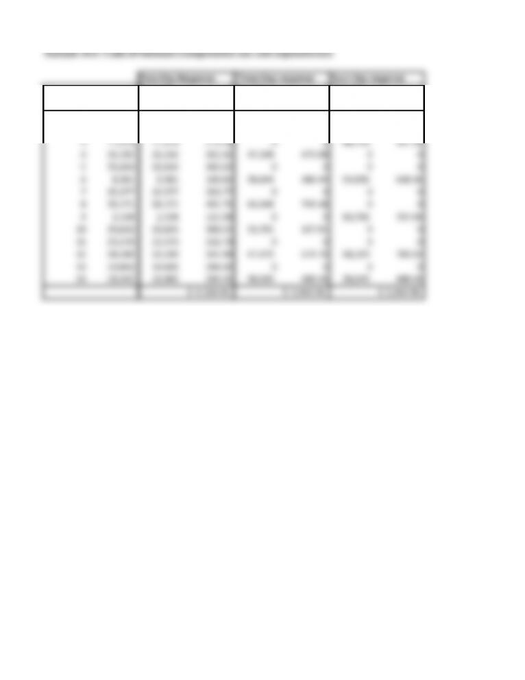
Example 14-4: Trade-off between transportation cost and responsiveness
Day Demand
Quantity
Shipped
Cost ($)
Quantity
Shipped
Cost ($)
Quantity
Shipped
Cost ($)
1 19,970 19,970 299.70 0 0 0 0
2 17,470 17,470 274.70 37,440 474.40 0 0
3 11,316 11,316 213.16 0 0 48,756 587.56
4 26,192 26,192 361.92 37,508 475.08 0 0
5 20,263 20,263 302.63 0 0 0 0
6 8,381 8,381 183.81 28,644 386.44 54,836 648.36
7 25,377 25,377 353.77 0 0 0 0
8 39,171 39,171 491.71 64,548 745.48 0 0
9 2,158 2,158 121.58 0 0 66,706 767.06
10 20,633 20,633 306.33 22,791 327.91 0 0
11 23,370 23,370 333.70 0 0 0 0
12 24,100 24,100 341.00 47,470 574.70 68,103 781.03
13 19,603 19,603 296.03 0 0 0 0
14 18,442 18,442 284.42 38,045 480.45 38,045 480.45
4,164.46$ 3,464.46$ 3,264.46$
Two-Day Response
Three-Day response
Four-Day response