Supply Chain Coordination with Commodity Products
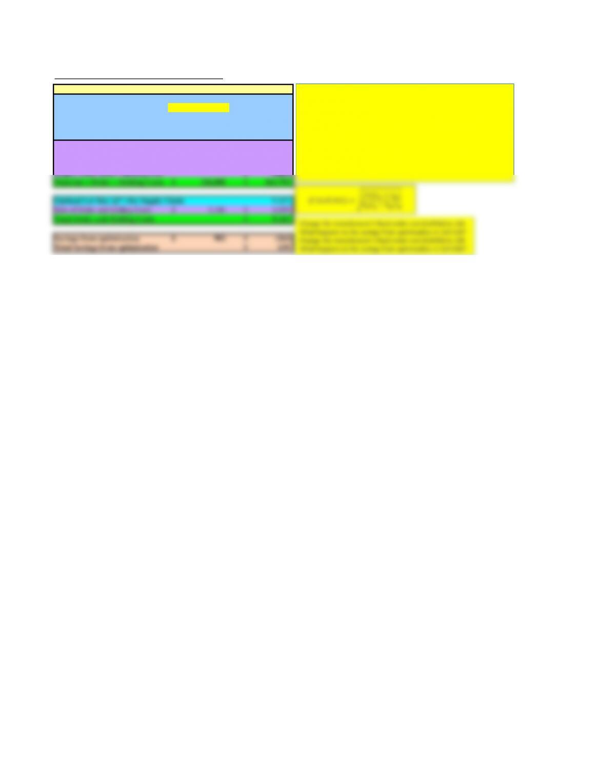
Manufacturer (M) DO (R )
Monthly Demand 10,000 10,000
Fixed Order Cost, S250$ 100$
Holding Cost, h20% 20%
Cost, C2.00$ 3.00$
Sale Price 3.00$
Calculated Lot Size 6,325
Sum of Order and Holding Cost 6,008$ 3,795$
Material Cost 240,000$ 360,000$
Supply Chain Order + Holding Cost
9,803$
Material + Order + Holding Costs 246,008$ 363,795$
Optimal Lot Size (Q* ) for Supply Chain 9,165
Sum of Order and holding Costs 5,106$ 4,059$
Total Order and Holding Costs 9,165$
Savings from optimization 902$ (264)$
Total Savings from optimization 638$
Cell D9 contains the order placed by DO when acting independently.
Cell B10 contains the manufacturer’s cost with this order size and
Cell D10 contains DO’s costs.
Cell D15 contains the optimal order size that minimizes manufacturer
plus DO’s costs, i.e., supply chain costs.
Cell B16 contains manufacturer’s costs and Cell D16 contains DO’s
costs with the supply chain optimal order size (Cell D15).
Cell B19 contains the manufacturer’s gains if DO orders supply chain
optimum. Cell D19 contains DO’s loss if DO orders supply chain optimum.
Cell D20 contains supply chain savings if DO orders supply chain optimum.
𝑄∗(𝐶𝑒𝑙𝑙 𝐷15) = 2𝐷(𝑆𝑅+ 𝑆𝑀)
ℎ𝑅𝐶𝑅+ ℎ𝑀𝐶𝑀
Change the manufacturer’s fixed order cost (Cell B5) to 150.
What happens to the savings from optimization in Cell D20?
Change the manufacturer’s fixed order cost (Cell B5) to 100.
What happens to the savings from optimization in Cell D20?
Designing a Suitable All Unit Discount
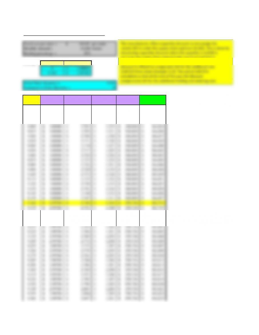
Fixed cost per order = 100.00$ per order
Monthly demand = 10,000 bottles
Holding percentage = 20%
Pricing: Min Quantity Price per sq. ft.
0 3.00000$
9,165 2.99780$
Order Average Annual Annual Annual Total
The manufacturer offers a quantity discount to encourage the
retailer DO to order the supply chain optimum (9,165). This is done by
structuring a quantity discount where the quantity in Cell B9 is
set to be the supply chain optimal order size from Cell D15 in
worksheet Example 11.9. For orders at or above this size, a
discount is offered to compensate DO for the additional cost
(Cell D19 from sheet Example 11.9). The cost in Cell C9 is
calculated so that at the end of the year the discount
9,375 2.99780$ 2,810$ 1,280$ 359,736$ 363,826$
9,385 2.99780$ 2,813$ 1,279$ 359,736$ 363,828$
9,395 2.99780$ 2,816$ 1,277$ 359,736$ 363,830$
Two Stage Supply Chain (With Market Power)
Manufacturer (M) DO (R)
Cost 2.00$ 4.00$
Sale Price 4.00$ 5.00$
Demand 60,000 60,000
Profit 120,000$ 60,000$
Total Profit = 180,000$
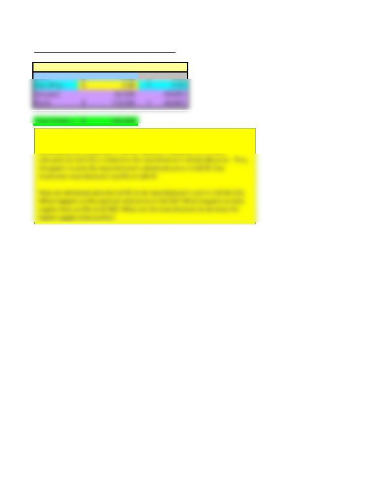
Demand curve is 360,000 – 60,000p for DO. Based on the retail price
in Cell D5, the resulting demand is shown in Cell D6. The manufacturer’s
wholesale price is selected in Cell B5. Based on Equation 11.15, DO’s
sale price (in Cell D5) is related to the manufacturer’s wholesale price. Thus,
the goal is to pick the manufacturer’s wholesale price in Cell B5 that
maximizes manufacturer’s profits in Cell B7.
Now set wholesale price in Cell B5 to be manufacturer’s cost in Cell B4 ($2).
What happens to the optimal retail price in Cell D5? What happens to total
supply chain profits (Cell B9)? What can the manufacturer to do keep the
higher supply chain profits?
Two Stage Supply Chain: 2-Part Tariff
Manufacturer (M) Retailer (R )
Cost 2.00$ 2.00$
Sale Price 2.00$ 4.00$
Franchise Fee (ff )180,000$
Demand 120,000 120,000
Profit 180,000$ 60,000$
Total Profit = 240,000$
Minimum Retailer Profit Required = 60,000$
2 Part Tariff
Demand curve is 360,000 – 60,000p for DO.
If Manufacturer sets wholesale price in Cell B5 to equal his cost in Cell B4, retail price
by DO is given in Cell D5. Once the wholesale price in Cell B5 is fixed to be $2
(manufacturer’s cost in Cell B4), the retailer DO sets the retail price inCell D5 to
maximize his profits (optimal retail price turns out to be $4).
Manufacturer can charge an up front franchise fee in Cell B6 (to extract all his profits
up front) while ensuring that DO gets at least the same profits he gets in Cell D7 of
sheet 2-stage when the two stages are not coordinated. Any franchise fee between
$120,000 and $180,000 will work. Total supply chain profits (Cell B10) are higher in
this case compared to the non-coordinated case.
Two Stage Supply Chain: Volume Based Discounts
Manufacturer (M) Retailer (R )
Purchase Price 2.00$ 3.50$
V1120,000
Sale Price 3.50$ 4.00$
C04.00$
Demand 120,000 120,000
C13.50$
Profit 180,000$ 60,000$
Total Profit = 240,000$
Minimum Retailer Profit Required = 60,000$
Volume Based Discounts
Demand curve is 360,000 – 60,000p for DO.
The goal here is to encourage the retailer to order an amount over
the year that maximizes supply chain profits. For the above demand
curve, this amount turns out to be 120,000 units. To sell 120,000
units, the retailer DO must set a retail price of $4 (Cell C5). The
manufacturer can set a unit price of $4 (Cell E5) for amounts below
120,000 units per year and lower the unit cost to any amount
between $ 3 and $3.50 (Cell E6) for amounts of 120,000 units or
more. The supply chain profit in this case is $240,000 with the
retailer making $60,000 (if Cell E6 is 3.50) or $120,000 (if Cell E6
is $3). As the manufacturer changes the discount price in Cell E6
from $3.50 down to $3.00, the distribution of profits changes.