Example 12-4
Inputs
Q D
s
Distribution of Demand during Lead Time
Cycle Service Level and Fill Rate
CSL ESC fr
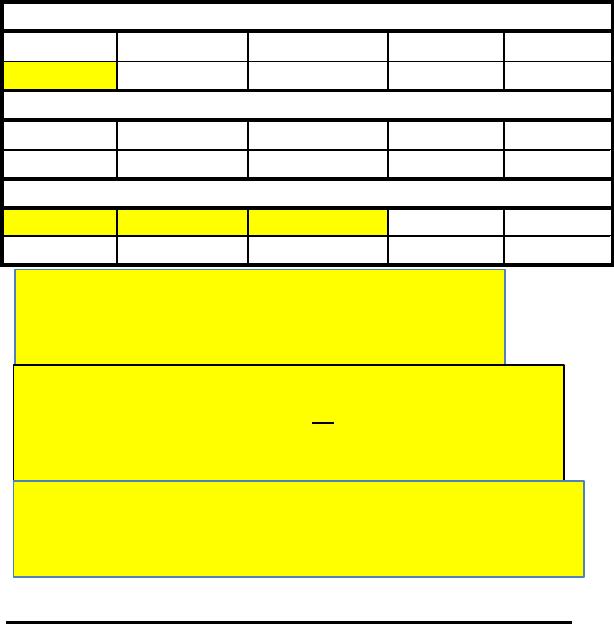
Evaluating Fill Rate Given Safety Inventory (Example 12-4)
Cell D9 using Equation 12.9
Fill Rate is calculated in Cell C9 using Equation 12.5
Change the batch size Qin Cell A3 and the safety inventory
in Cell E3 to see how it impacts the CSL (Cell A9) and the
fill rate fr (Cell C9)
Page 12
Example 12-5
Calculation Variable
fr
σLQ Desired ESC ss
Input
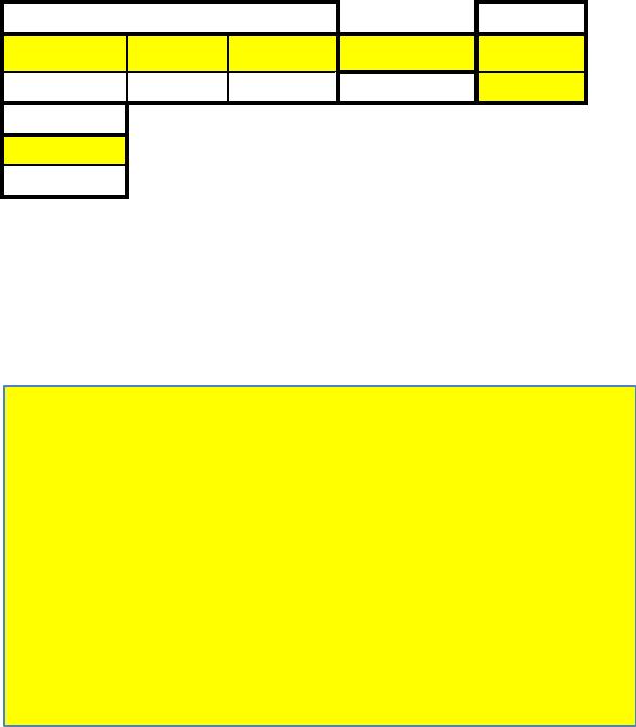
To manually estimate the safety stock, change the value in
Cell E3 until the value in Cell A6 equals that in Cell D3.
To use GoalSeek, proceed as follows:
Repeat the process for different values of fill rate fr in Cell A3
to build Table 12-1.
Impact of Reducing Lead Time and Forecast Error (Example 12-6)
Input
Demand per period (week), D = 2500 shirts
Desired cycle service level, CSL = 0.95
Solution
Required safety inventory, ss = 3,948
Change standard deviation of demand in Cell D4
Example 12-7
Evaluating the Impact of Lead Time Uncertainty on Safety Inventory (Example 12-7)
Input
Demand per period (day), D = 2500
Avg. replenishment lead time, L = 7 days
Solution
Intermediate Calculation
Resulting Safety Inventory Level
Estimated safety inventory (units), ss = 22,491
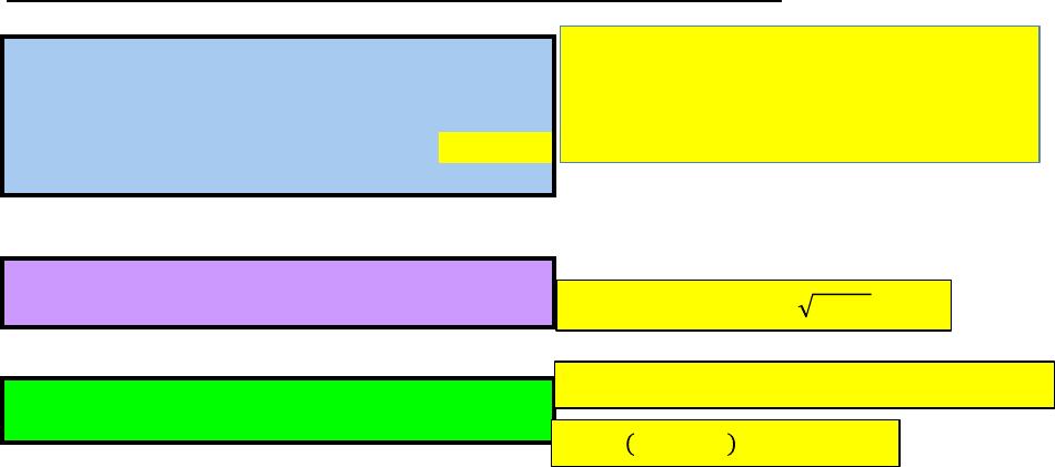
Cell E12 is calculated using Equation 12.11.
𝜎𝐿
(
𝐶𝑒𝑙𝑙 𝐸12
)
= 𝐿𝜎𝐷2+ 𝐷2𝑠𝐿2
Example 12-8
Value of Aggregation (Example 12-8)
Demand per period (weekly) per location, D (cars)= 25
Desired cycle service level, CSL = 0.90
Number of retail outlets 4
Cost per Vehicle 20,000$
Intermediate calculation
Disaggregate
Option
Aggregate Option
Mean Weekly Demand, DC100
# of weeks’ demand = 1.45 0.72
Annual Holding Cost Savings 72,496$
Cell E22 contains safety inventory on aggregation while
Cell D22 contains safety inventory on disaggregation.
Example 12-9
Trade-offs of Physical Aggregation (Example 12-9)
Demand per period (weekly) per location, D (cars)= 1000
Standard deviation of demand,
s
D = 300
Desired cycle service level, CSL = 0.95
Number of retail outlets 4
Cost per unit 1,000$
Intermediate Calculation
Disaggregate
Option
Aggregate Option
Mean Weekly Demand, DC4000
Standard Deviation of demand, sD
Mean demand during lead time DL =
Resulting Safety Inventory Level at Each Retail Outlet
Total Safety Inventory Required
# of weeks’ demand = 3.95 1.97
Safety Inventory Savings through Aggregation
Annual Holding Cost Savings on Aggregation 394,765$
Change in Operating and Transportation Cost
Operating cost decrease on aggregation 150,000$
Transportation cost/unit 10$ 13$
Increase in transportation cost on aggregation 624,000$
Total increase in operating and transportation cost on aggregation 474,000$
Cell E28 contains the holding cost savings on aggregation.
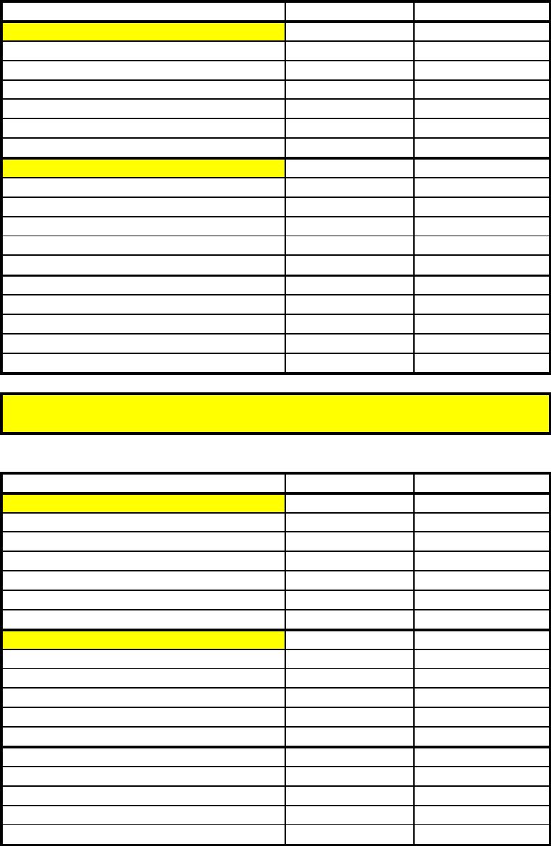
Example 12-10 Impact of Coefficient of Variation on Value of Aggregation
Motors Cleaner
Inventory Is Stocked in Each Store
Mean weekly demand per store 20 1,000
Inventory Is Aggregated at DC
Mean weekly aggregate demand 32,000 1,600,000
Savings
Total inventory saving on aggregation 102,638,866$ 15,395,830$
The numbers above are slightly different from the numbers in Table 12-4 because
inventory values are not rounded (in the book they are rounded).
Rounded Numbers as Shown in Table 12-4
Motors Cleaner
Inventory Is Stocked in Each Store
Mean weekly demand per store 20 1,000
Standard deviation 40 100
Inventory Is Aggregated at DC
Mean weekly aggregate demand 32,000 1,600,000
Standard deviation of aggregate demand 1,600 4,000
Savings
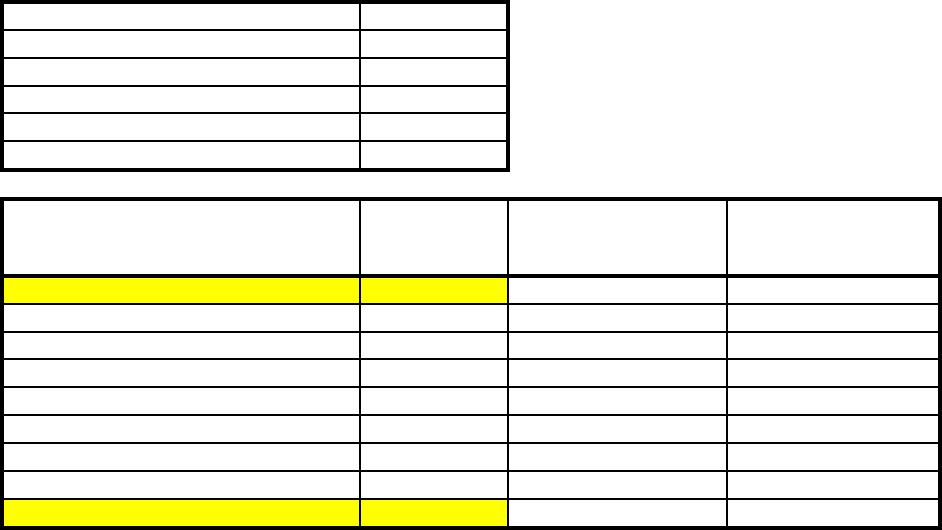
Example 12-11 Value of Component Commonality
Mean demand per server 5000
Standard deviation of demand 3000
Replenishment lead time 1
Number of Finished Products per
Component
Safety
Inventory
Marginal Reduction in
Safety Inventory
Total Reduction in
Safety Inventory
1 399,699
2 282,630 117,069 117,069
3 230,767 51,864 168,933
Value of Postponement (Example 12-12)
Demand per period (weekly) per color, D = 30
Standard deviation of demand, sD = 10
Avg replenishment lead time, L (weeks)= 2
Desired cycle service level, CSL = 0.95
Intermediate Calculation
Without
Postponement
With
Postponement
Mean Weekly Demand, DC3000
Standard Deviation of demand, sD
C100
Mean demand during lead time DL = 60 6000
Resulting Safety Inventory Level for Each Color
Estimated safety inventory (units) = 23.26 0
Total Safety Inventory Required
# of weeks’ demand = 77.54 7.75
Safety Inventory Savings through Postponement
Unit Savings 2094
Example 12-13
Evaluating Safety Inventory for Periodic Review Policies (Example 12-13)
Input
Demand per period (week), D (boxes) = 2500
Replenishment lead time, L (weeks)= 2
Review interval, T (weeks)= 4
Cell D14 is calculated using Equation 12.19
Cell D15 is calculated using Equation 12.18
Page 21
Example 12-13
Page 22