16 ADJUSTMENT BY LEAST SQUARES
Asterisks (*) indicate problems that have partial answers given in Appendix G.
16.1 What fundamental condition is enforced by the method of weighted least squares?
16.8 In Problem 16.6, the standard deviations of the three angles are ±2.5″, ±1.0″, and ±1.9″
respectively. What are the most probable values for the three angles?
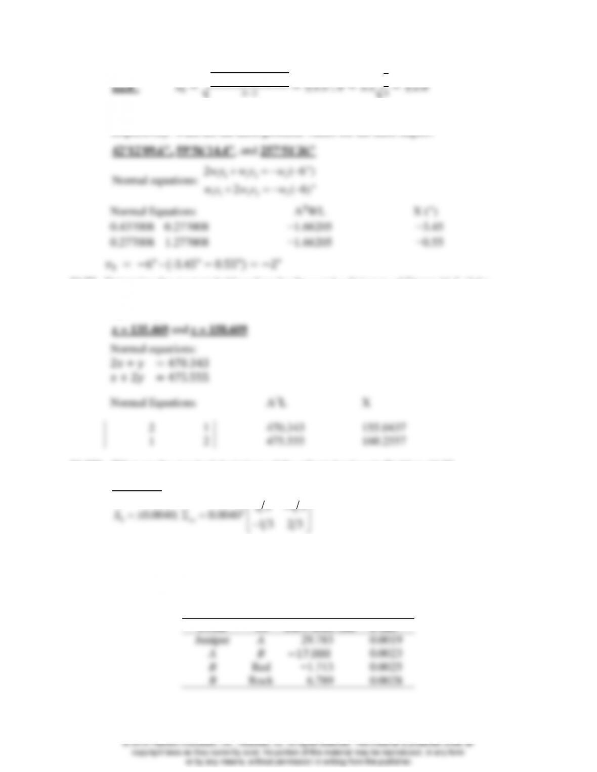
16.9* Determine the most probable values for the x and y distances of Figure 16.2, if the
observed lengths of AC, AB, and BC (in meters) are 315.297, 155.046, and 160.258,
respectively.
685.673 29.783 715.456
17.000
696.745 1.713 698.458
705.253 6.789 698.464
A
AB
B
B
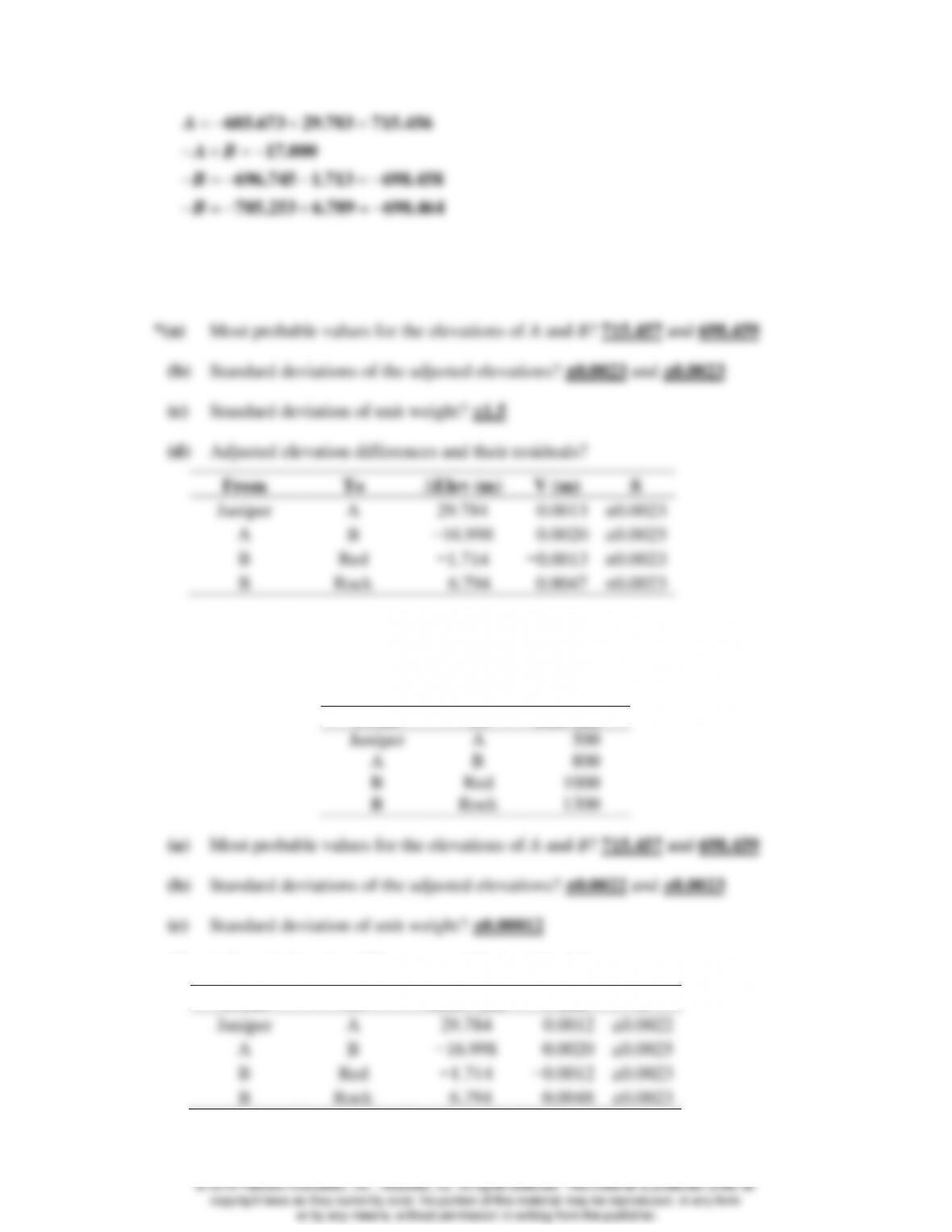
16.12 For Problem 16.11, following steps outlined in Example 16.6 perform a weighted least–
squares adjustment of the network. Determine weights based upon the given standard
deviations. What are the
From
To
∆Elev (m)
V (m)
S
Juniper
A
29.784
0.0013
±0.0023
A
B
−16.998
0.0020
±0.0025
B
Red
−1.714
−0.0013
±0.0023
B
Rock
6.794
0.0047
±0.0023
(e) Standard deviations of the adjusted elevation differences? (See part d)
16.13 Repeat Problem 16.12 using distances for weighting. Assume the following course
lengths for the problem.
From
To
Dist (m)
Juniper
A
500
A
B
800
B
Red
1000
B
Rock
1300
(a) Most probable values for the elevations of A and B? 715.457 and 698.459
(b) Standard deviations of the adjusted elevations? ±0.0022 and ±0.0023
(c) Standard deviation of unit weight? ±0.00012
(d) Adjusted elevation differences and their residuals?
From
To
∆Elev (m)
V (m)
S
Juniper
A
29.784
0.0012
±0.0022
A
B
−16.998
0.0020
±0.0025
B
Red
−1.714
−0.0012
±0.0023
B
Rock
6.794
0.0048
±0.0023
© 2018 Pearson Education, Inc., Hoboken, NJ. All rights reserved. This material is protected under all
copyright laws as they currently exist. No portion of this material may be reproduced, in any form
or by any means, without permission in writing from the publisher.
(e) Standard deviations of the adjusted elevation differences? (See d)
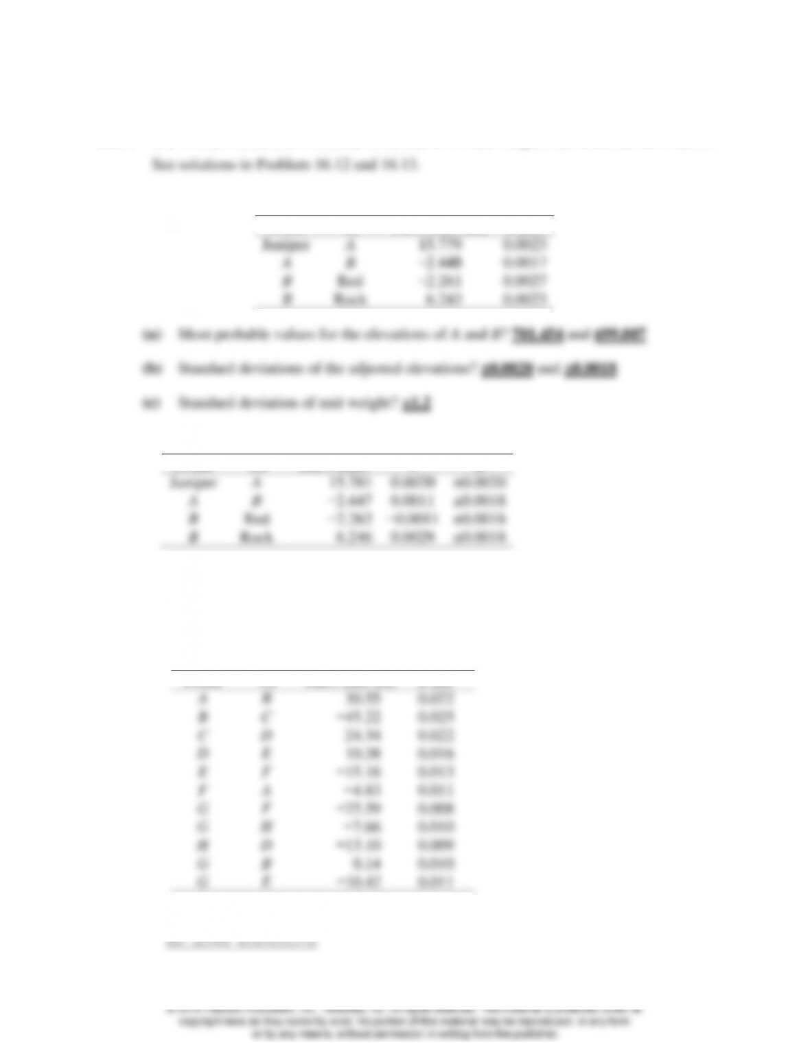
16.14 Use WOLFPACK to do Problem 16.12 and 16.13 and compare the solutions for A and B.
16.15 Repeat Problem 16.12 using the following data.
From
To
Elev. Diff. (m)
σ (m)
Juniper
A
15.779
0.0023
A
B
−2.448
0.0017
B
Red
−2.261
0.0027
B
Rock
6.243
0.0023
(a) Most probable values for the elevations of A and B? 701.454 and 699.007
(b) Standard deviations of the adjusted elevations? ±0.0020 and ±0.0018
(c) Standard deviation of unit weight? ±1.2
(d) Adjusted elevation differences and their residuals?
From
To
Elev. Diff.
V
S
Juniper
A
15.781
0.0020
±0.0020
A
B
−2.447
0.0011
±0.0018
B
Red
−2.262
−0.0011
±0.0018
B
Rock
6.246
0.0029
±0.0018
(e) Standard deviations of the adjusted elevation differences? (See d)
16.16 A network of differential levels is shown in the accompanying figure. The elevations of
benchmarks A and G are 835.24 ft and 865.64 ft, respectively. The observed elevation
differences and the distances between stations are shown in the following table. Using
WOLFPACK, determine the
From
To
Elev. Diff (ft)
S (ft)
A
B
30.55
0.022
B
C
−45.22
0.025
C
D
24.34
0.022
D
E
10.38
0.016
E
F
−15.16
0.013
F
A
−4.83
0.011
G
F
−25.59
0.008
G
H
−7.66
0.010
H
D
−13.10
0.009
G
B
0.14
0.010
G
E
−10.42
0.011
(a) Most probable values for the elevations of new benchmarks B, C, D, E, F, and H?
(b) Standard deviations of the adjusted elevations? See (a)
(c) Standard deviation of unit weight? 1.2
(d) Adjusted elevation differences and their residuals?
Adjusted Elevation Differences
From To Elevation Difference V S
────────────────────────────────────────────────────
(e) Standard deviations of the adjusted elevation differences? See (d).
16.17 Develop the observation equations for line AB and BC in Problem 16.16.
16.18 A network of GNSS observations shown in the accompanying figure was made with two
receivers using the static method. Known coordinates of the two control stations are in
the geocentric system. Develop the observation equations for the following baseline
vector components.
1
2
3
4
5
6
1,646,897.428
4,212,279.218
4,482,199.783
1,646,897.432
4,212,279.215
4,452,199.779
Troy
Troy
Troy
Troy
Troy
Troy
Xv
Yv
Zv
Xv
Yv
Zv
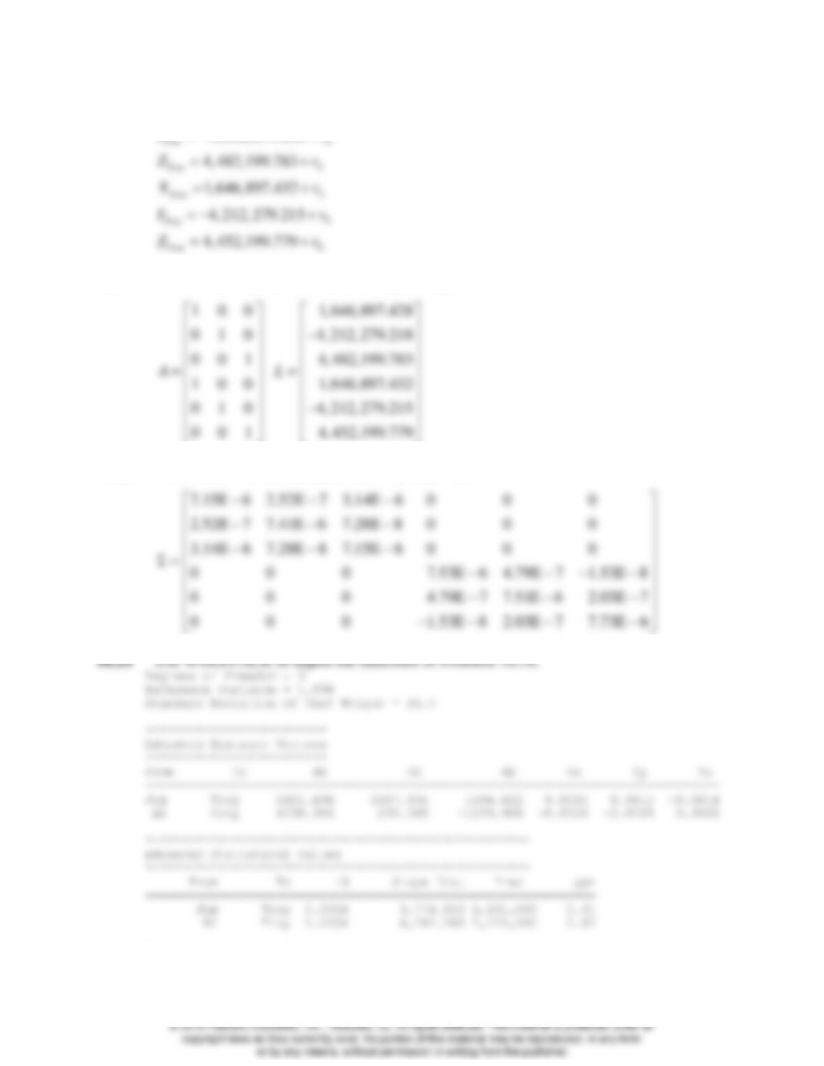
16.19 For Problem 16.18, construct the A and L matrices.
1 0 0 1,646,897.428
0 1 0 4,212,279.218
0 0 1 4,482,199.783
1 0 0 1,646,897.432
0 1 0 4,212,279.215
0 0 1 4,452,199.779
AL
16.20 For Problem 16.18, construct the covariance matrix.
7.15E 6 2.52E 7 3.14E 6 0 0 0
2.52E 7 7.41E 6 7.28E 8 0 0 0
3.14E 6 7.28E 8 7.15E 6 0 0 0
0 0 0 7.53E 6 4.79E 7 1.53E 8
0 0 0 4.79E 7 7.51E 6 2.03E 7
0 0 0 1.53E 8 2.03E 7 7.73E 6
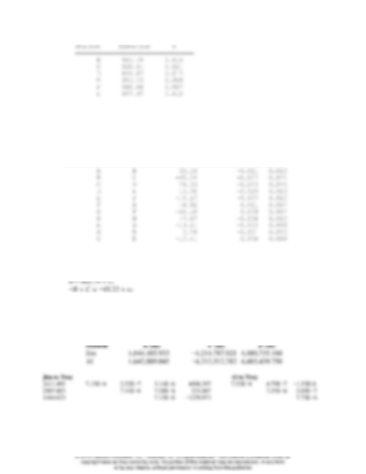
16.21 Use WOLFPACK to adjust the baselines of Problem 16.18.
Degrees of Freedom = 3
Reference Variance = 1.096
Standard Deviation of Unit Weight = ±1.0
*************************
Adjusted Distance Vectors
*************************
From To dX dY dZ Vx Vy Vz
===============================================================================
Jim Troy 2411.496 2507.804 1464.622 0.0014 0.0015 -0.0014
Al Troy 4008.384 233.065 -1239.968 -0.0026 -0.0015 0.0026
*****************************************************
Advanced Statistical Values
*****************************************************
From To ±S Slope Dist Prec ppm
==============================================================
Jim Troy 0.0034 3,774.853 1,101,000 0.91
Al Troy 0.0034 4,202.260 1,225,000 0.82

16.22 Convert the geocentric coordinates obtained for station Troy in Problem 16.21 to geodetic
coordinates using the WGS84 ellipsoidal parameters.
16.23 A network of GNSS observations shown in the accompanying figure was made with two
receivers using the static method. Use WOLFPACK to adjust the network, given the
following data.
Station
X (m)
Y (m)
Z (m)
Bonnie
−2,660,581.015
−1,513,935.768
5,576,785.765
Tom
−2,648,294.114
−1,526,048.226
5,579,322.060
Bonnie to Ray
Bonnie to Herb
−3,886.055
3.06E−5
−1.04E−7
6.28E−7
10,207.052
1.68E−5
7.85E−7
3.15E−7
−15,643.129
3.14E−5
6.86E−7
−2,006.464
1.93E−5
4.63E−7
−6,079.276
3.06E−5
4,295.068
1.70E−5
Tom to Ray
Tom to Herb
−16,172.951
3.43E−5
1.64E−6
4.06E−7
−2,079.844
1.51E−5
3.78E−7
−1.90E−6
−3,530.664
3.49E−5
7.71E−7
10,105.996
1.51E−5
1.45E−6
−8,615.580
3.68E−5
1,758.774
1.54E−5
Bonnie to Tom (Fixed line—Don’t use in adjustment.)
12,286.899
3.21E−5
−6.99E−7
1.20E−6
−12,112.451
3.11E−5
6.65E−7
2,536.295
3.21E−5
Degrees of Freedom = 9
Reference Variance = 0.5519
Standard Deviation of Unit Weight = ±0.74
*************************
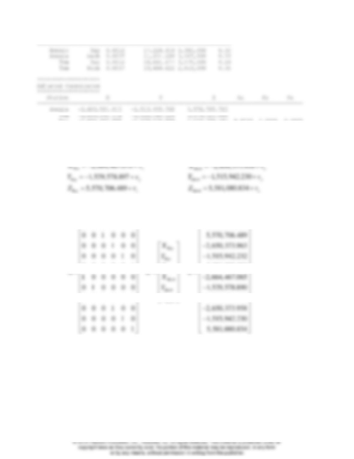
Ray -2,664,467.068 -1,529,578.894 5,570,706.485 0.0030 0.0030 0.0030
Herb -2,650,373.960 -1,515,942.231 5,581,080.834 0.0021 0.0022 0.0021
16.24 For Problem 16.23, write the observation equations for the baselines “Bonnie to Ray” and
“Tom to Herb.”
2,664,467.070
1,529,578.897
5,570,706.489
Ray x
Ray y
Ray z
Xv
Yv
Zv
2,650,373.958
1,515,942.230
5,581,080.834
Herb x
Herb y
Herb z
Xv
Yv
Zv
16.25 For Problem 16.23, construct the A, X, and L matrices for the observations.
1 0 0 0 0 0 2,664,467.070
0 1 0 0 0 0 1,529,578.897
0 0 1 0 0 0 5,570,706
0 0 0 1 0 0
0 0 0 0 1 0
0 0 0 0 0 1
1 0 0 0 0 0
0 1 0 0 0 0
0 0 1 0 0 0
0 0 0 1 0 0
0 0 0 0 1 0
0 0 0 0 0 1
Ray
Ray
Ray
Herb
Herb
Herb
X
Y
Z
A X L
X
Y
Z
.489
2,650,373.963
1,515,942.232
5,581,080.833
2,664,467.065
1,529,578.890
5,570,706.480
2,650,373.958
1,515,942.230
5,581,080.834
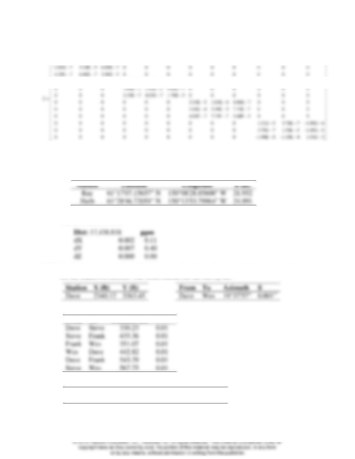
16.26 For Problem 16.23, construct the covariance matrix.
3.06E 5 1.04E 7 6.28E 7 0 0 0 0 0 0 0 0 0
1.04E 7 3.14E 5 6.86E 7 0 0 0 0 0 0 0 0 0
6.28E 7 6.86E 7 3.06E 5 0 0 0 0 0 0 0 0 0
0 0 0 1.68E 5 7.85E 7 3.15E 7 0 0 0 0 0 0
0 0 0 7.85E 7 1.93E 5 4.63E 7 0 0 0 0 0 0
0 0 0 3.15E 7 4.63E 7 1.70E 5 0 0 0 0 0 0
0 0 0 0 0 0 3.43E 5 1.6
4E 6 4.06E 7 0 0 0
0 0 0 0 0 0 1.64E 6 3.49E 5 7.71E 7 0 0 0
0 0 0 0 0 0 4.06E 7 7.71E 7 3.68E 5 0 0 0
0 0 0 0 0 0 0 0 0 1.51E 5 3.78E 7 1.90E 6
0 0 0 0 0 0 0 0 0 3.78E 7 1.51E 5 1.45E 6
0 0 0 0 0 0 0 0 0 1.90E 6 1.45E 6 1.54E 5
16.27* After completing Problem 16.23, convert the geocentric coordinates for station Ray and
Herb to geodetic coordinates using the WGS84 ellipsoidal parameters. (Hint: See Section
13.4.3)
Station
Latitude
Longitude
h (m)
Ray
61°17’07.15657″ N
150°08’28.85600″ W
21.952
Herb
61°28’46.72051″ N
150°13’53.79964″ W
24.991
16.28 Following the procedures discussed in Section 14.5.2, analyze the fixed baseline from
station Bonnie to Tom.
Dist: 17,438.818
ppm
dX
0.002
0.11
dY
0.007
0.40
dZ
0.000
0.00
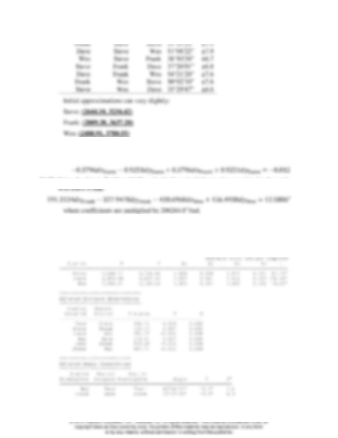
16.29 For the horizontal survey of the accompanying figure, determine initial approximations
for the unknown stations. The observations for the survey are
Station
X (ft)
Y (ft)
From
To
Azimuth
S
Dave
2340.12
3363.45
Dave
Wes
19°37′57″
0.001”
From
To
Distance (ft)
Dave
Steve
330.23
0.01
Steve
Frank
435.36
0.01
Frank
Wes
351.07
0.01
Wes
Dave
442.82
0.01
Dave
Frank
543.29
0.01
Steve
Wes
567.75
0.01
Station
Station
Station
Angle
σ″
(ft)
Frank
Dave
Steve
53°15′24″
±7.9
Dave
Steve
Wes
51°08′22″
±7.9
Wes
Steve
Frank
38°10′30″
±6.7
Steve
Frank
Dave
37°26′01″
±6.8
Dave
Frank
Wes
54°21′20″
±7.6
Frank
Wes
Steve
50°02′10″
±7.6
Steve
Wes
Dave
35°29′47″
±6.6
Initial approximations can vary slightly:
Steve: (2644.10, 3234.42)
Frank: (2809.38, 3637.20)
Wes: (2488.91, 3780.55)
16.30* Using the data in Problem 16.29, write the linearized observation equation for the distance
from Steve to Frank.
16.31 Using the data in Problem 16.29, write the linearized observation equation for the angle
16.32 Assuming a standard deviation of ±0.001” for the azimuth line Dave-Wes, use
WOLFPACK to adjust the data in Problem 16.29.
*****************
Adjusted stations
*****************
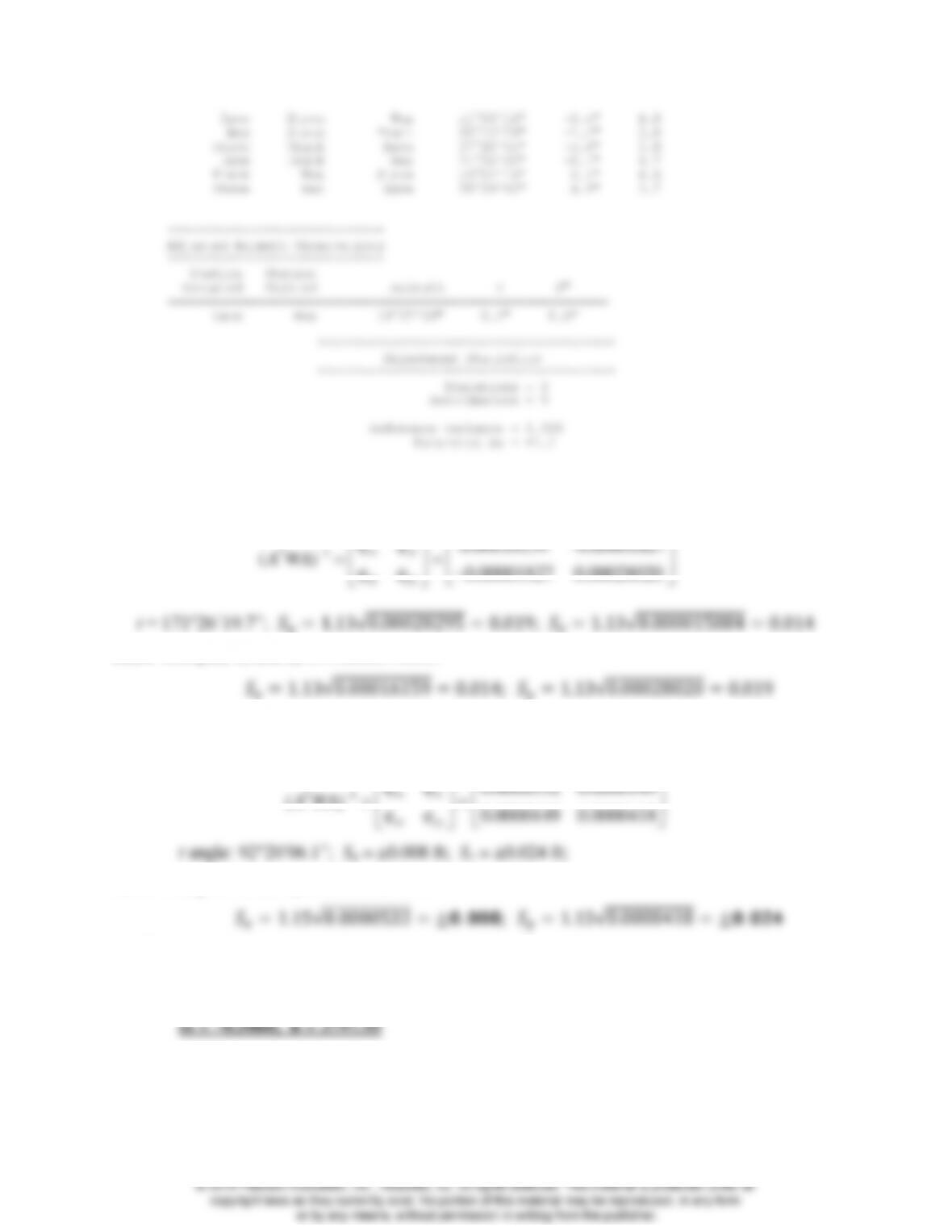
16.33* Given the following inverse matrix and a standard deviation of unit weight of 1.13,
determine the parameters of the error ellipse.
10.00016159 –0.00001827
( )
0.00001827 0.00028020
xx xy
T
xy yy
qq
A WA qq
t = 171°26’19.7”; 𝑆𝑢= 1.13√0.00028295 = 0.019; 𝑆𝑣= 1.13√0.000015884 = 0.014
16.34 Compute Sx and Sy in Problem 16.33.
16.35 Given the following inverse matrix and a standard deviation of unit weight of 1.15,
determine the parameters of the error ellipse.
10.0000532 0.0000149
() 0.0000149 0.0000418
xx xy
T
xy yy
qq
A WA qq
16.36 Compute Sx and Sy in Problem 16.35.
16.37 The well-known observation equation for a line is mx + b = y + vy. What is the slope and
y-intercept of the best fit line for a set of points with coordinates (1446.81, 2950.79),
(2329.79, 2432.66), (3345.74, 1837.13), (478.72, 3517.64), (4382.98, 1229.16)?
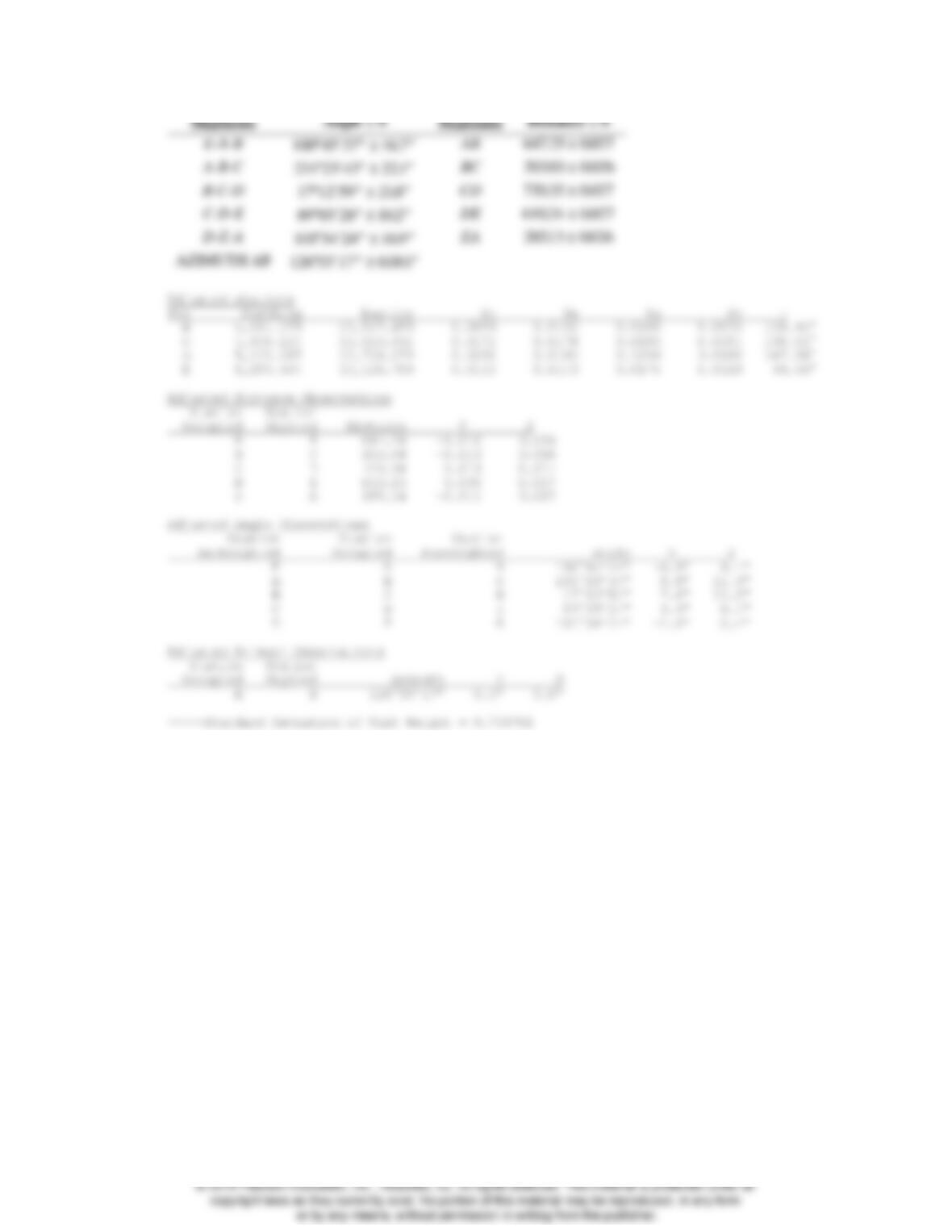
16.38 Use WOLFPACK and the following standard deviations for each observation to do a least
squares adjustment of Example 10.4, and describe any differences in the solution. What
advantages are there to using the least squares method in adjusting this traverse?
© 2018 Pearson Education, Inc., Hoboken, NJ. All rights reserved. This material is protected under all
Stations
Stations
E-A-B
AB
A-B-C
BC
B-C-D
CD
C-D-E
DE
D-E-A
EA
AZIMUTH AB
Adjusted stations
Sta Northing Easting Sn Se Su Sv t
B 4,611.179 10,517.459 0.0099 0.0132 0.0165 0.0000 126.92°
C 4,408.224 10,523.432 0.0172 0.0178 0.0193 0.0154 130.51°
D 5,102.267 10,716.279 0.0232 0.0192 0.0256 0.0160 147.58°
E 5,255.934 10,125.709 0.0150 0.0149 0.0175 0.0119 44.56°
Adjusted Distance Observations
Station Station
Occupied Sighted Distance V S
A B 647.26 –0.010 0.016
B C 203.04 –0.013 0.016
C D 720.34 0.013 0.017
D E 610.23 0.005 0.017
E A 285.14 –0.011 0.017
Adjusted Angle Observations
Station Station Station
Backsighted Occupied Foresighted Angle V S
E A B 100°45’44” –6.9” 9.1”
A B C 231°23’34” 8.8” 12.3”
B C D 17°12’51” 7.6” 10.2”
C D E 89°03’24” 4.4” 6.1”
D E A 101°34’27” –2.9” 8.4”
Adjusted Azimuth Observations
Station Station
Occupied Sighted Azimuth V S
A B 126°55’17” 0.0” 0.0”
—–Standard Deviation of Unit Weight = 0.700781
Angle S
Distance S
100 45 37 167
.
647 25 0027. .
231 23 43 221
.
20303 0026. .
17 12 59 218
.
72035 0027. .
89 03 28 102
.
61024 0027. .
101 34 24 169
.
28513 0026. .
126 55 17 0001
.
© 2018 Pearson Education, Inc., Hoboken, NJ. All rights reserved. This material is protected under all
copyright laws as they currently exist. No portion of this material may be reproduced, in any form
or by any means, without permission in writing from the publisher.

© 2018 Pearson Education, Inc., Hoboken, NJ. All rights reserved. This material is protected under all