


-15.0%
-10.0%
-5.0%
0.0%
5.0%
10.0%
15.0%
20.0%
25.0%
30.0%
35.0%
40.0%
-13.0% -8.0% -4.0% 0.0% 2.0% 6.0% 8.0% 10.0% 13.0% 15.0% 16.0%
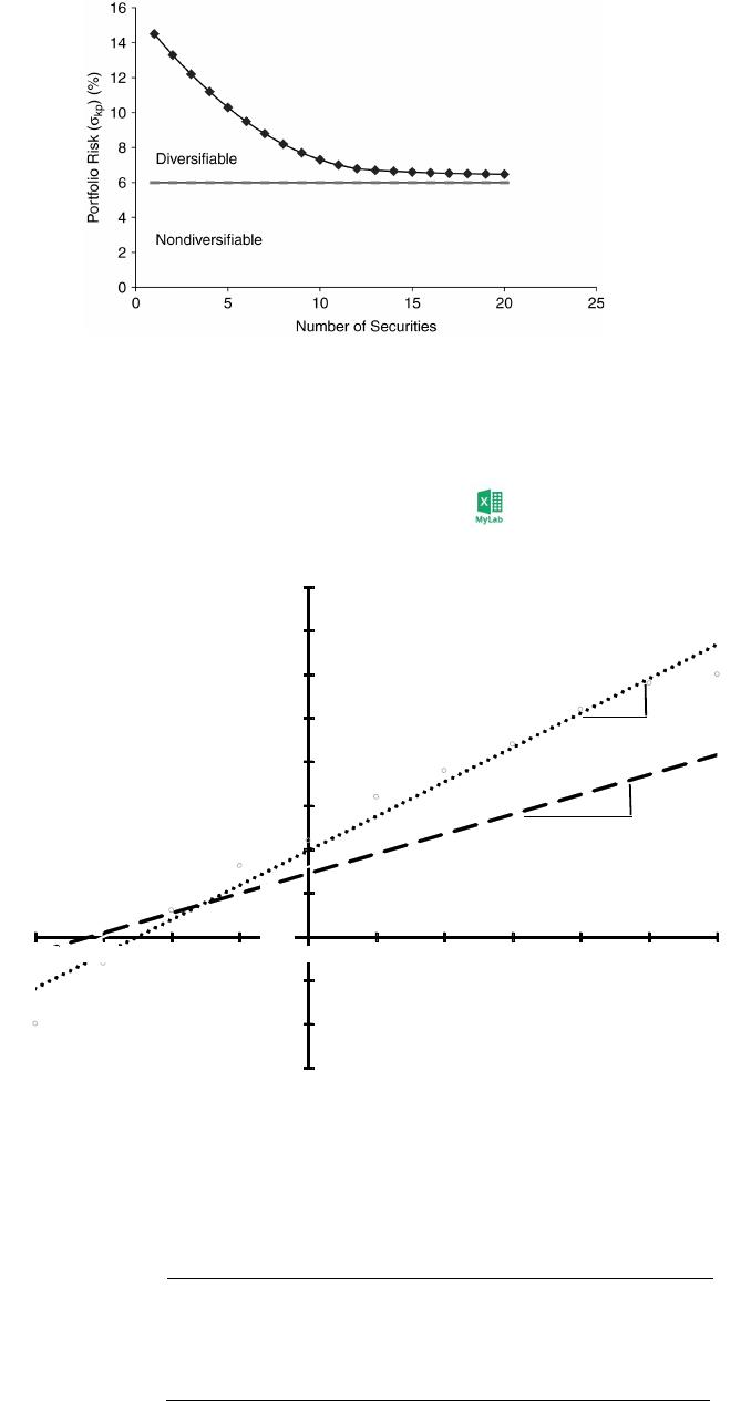
Deriving Beta
Asset B
Beta = 1.38
Asset A
Beta = 0.793
Asset
Returns
Market
Return
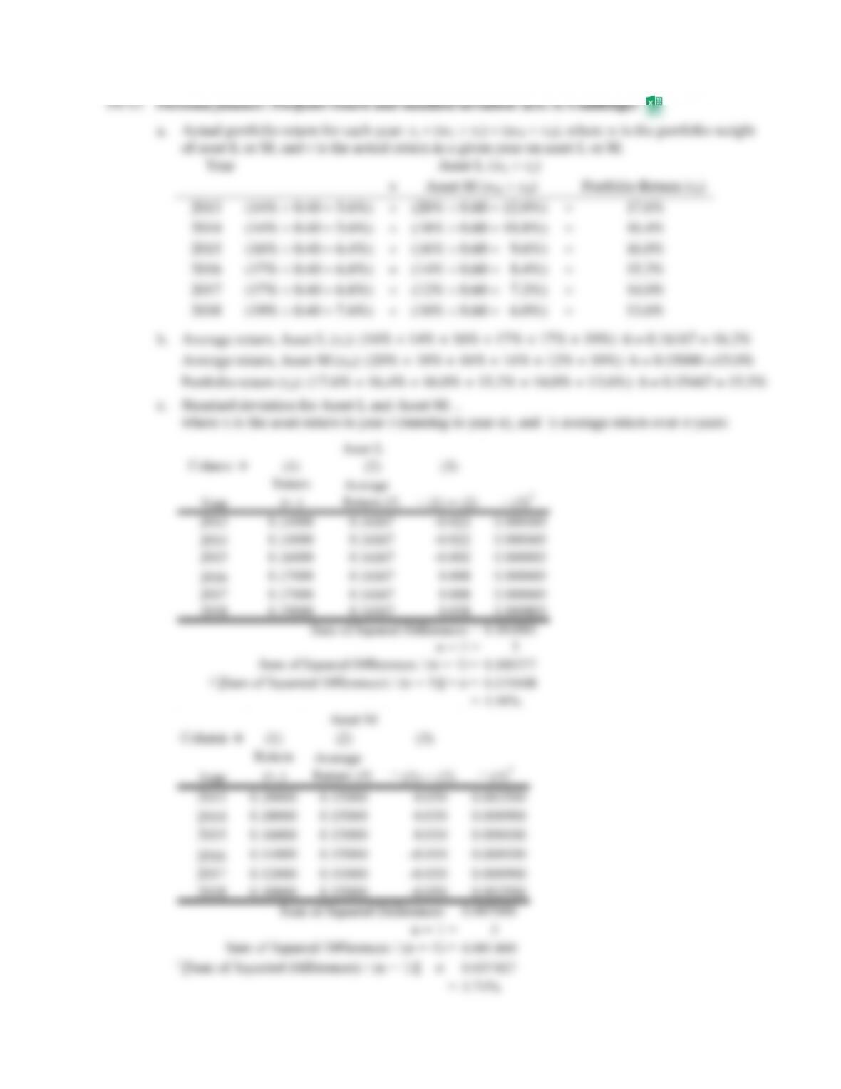
P8-17 Total, non-diversifiable, and diversifiable risk (LG 5; Intermediate)
a. and b.
c. Only nondiversifiable risk is relevant because, as shown above, building a portfolio of at least
20 securities with imperfectly correlated returns substantially reduces diversifiable risk. When
additional securities no longer reduce risk, the remaining standard deviation of David Talbot’s
portfolio is non-diversifiable. That standard deviation of returns of 6.47% (down from 14.50%).
P8-18 Graphic derivation of beta (LG 5; Intermediate)
a.
b. The betas for assets A and B are the slopes of the characteristic lines above. Typically, the
slopes of these lines are estimated with a statistical technique known as linear regression. But,
slope can also be calculated given any two points on a line. Here, we can obtain slopes (i.e.,
betas) with the highest and lowest returns for each asset. Specifically:
Beta = ∆ Asset Return ∆ Market Return
BetaAsset A = Highest Return on Asset A – Lowest Return on Asset A
Highest Market Return – Lowest Market Return
= [0.19 – (–0.04)] [0.16 – (–0.13)] = 0.23 0.29 = 0.793
BetaAsset B = Highest Return on Asset B – Lowest Return on Asset B
Highest Market Return – Lowest Market Return