
Market
Expected Return
Weighted Value


Return Probability Weighted Value
r
i
P
ri
r
i
x P
ri
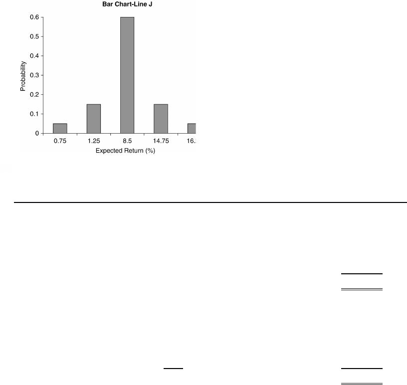
-0.10 0.010 -0.001000
0.10 0.040 0.004000
0.20 0.050 0.010000
0.30 0.100 0.030000
0.40 0.150 0.060000
0.45 0.300 0.135000
0.50 0.150 0.075000
0.60 0.100 0.060000
0.70 0.050 0.035000
0.80 0.040 0.032000
1.00 0.010 0.010000
Sum = 1.000
Sum = Average Return (r
r) = 0.450000
= 45.0%
(3) Standard deviation: , where:
ri is the return for outcome i, is the average return across all outcomes, and Pri is the
probability of outcome i.
Column → (1) (2) (3) (4) (5) (6)
Return
(r
i
)
Average
Return (r
r)
= (1) ─ (2) = (3)
2
Probability
(P
ri
)
= (4) x (5)
-0.10 0.45 -0.550 0.3025 0.010 0.003025
0.10 0.45 -0.350 0.1225 0.040 0.004900
0.20 0.45 -0.250 0.0625 0.050 0.003125
0.30 0.45 -0.150 0.0225 0.100 0.002250
0.40 0.45 -0.050 0.0025 0.150 0.000375
0.45 0.45 0.000 0.0000 0.300 0.000000
0.50 0.45 0.050 0.0025 0.150 0.000375
0.60 0.45 0.150 0.0225 0.100 0.002250
0.70 0.45 0.250 0.0625 0.050 0.003125
0.80 0.45 0.350 0.1225 0.040 0.004900
1.00 0.45 0.550 0.3025 0.010 0.003025
Sum = 0.027350
0.16538
= 16.54%
√ (Sum) = Standard Deviation (σ) =
(4) Coefficient of variation (CV) is given by σ , where σ is the standard deviation of returns on
the asset and is the average return. So:
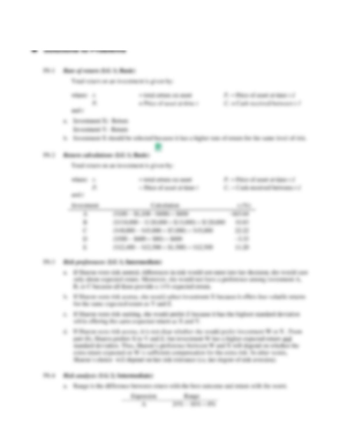
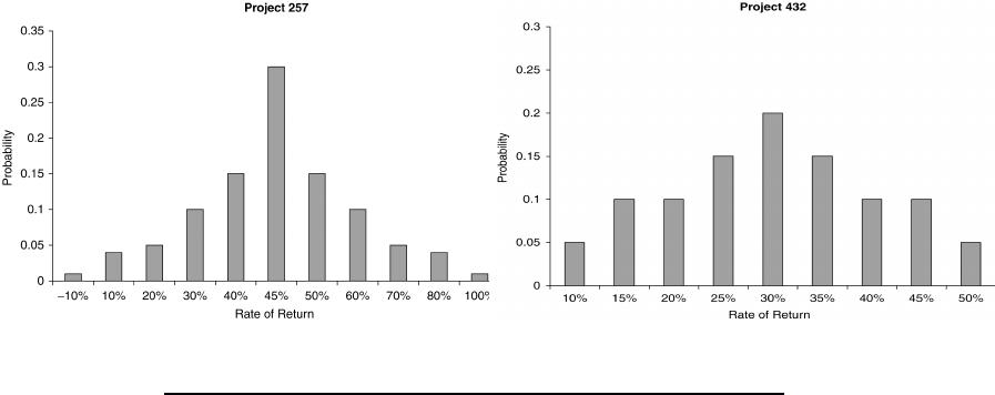
Project 432

Return Probability Weighted Value
r
i
P
ri
r
i
x P
ri
0.10 0.050 0.0050
0.15 0.100 0.0150
0.20 0.100 0.0200
0.25 0.150 0.0375
0.30 0.200 0.0600
0.35 0.150 0.0525
0.40 0.100 0.0400
0.45 0.100 0.0450
0.50 0.050 0.0250
Sum = 1.000
Sum = Average Return (r
r) = 0.300000
= 30.0%
(3) Standard deviation: , where:
ri is the return for outcome i, is the average return across all outcomes, and Pri is the
probability of outcome i.
Column → (1) (2) (3) (4) (5) (6)
Return
(r
i
)
Average
Return (r
r)
= (1) ─ (2) = (3)
2
Probability
(P
ri
)
= (4) x (5)
0.10 0.30 -0.200 0.0400 0.050 0.002000
0.15 0.30 -0.150 0.0225 0.100 0.002250
0.20 0.30 -0.100 0.0100 0.100 0.001000
0.25 0.30 -0.050 0.0025 0.150 0.000375
0.30 0.30 0.000 0.0000 0.200 0.000000
0.35 0.30 0.050 0.0025 0.150 0.000375
0.40 0.30 0.100 0.0100 0.100 0.001000
0.45 0.30 0.150 0.0225 0.100 0.002250
0.50 0.30 0.200 0.0400 0.050 0.002000
Sum = 0.011250
0.106066
= 10.61%
√ (Sum) = Standard Deviation (σ) =
(4) Coefficient of variation (CV) is given by σ , where σ is the standard deviation of returns on
the asset and is the average return. So: CV = 0.106066 0.300 = 0.3536.


Asset F
Column → (1) (2) (3) (4) (5) (6)
Return
(r
i
)
Average
Return (r
r)
= (1) ─ (2) = (3)
2
Probability
(P
ri
)
= (4) x (5)
0.40 0.04 0.360 0.1296 0.100 0.012960
0.10 0.04 0.060 0.0036 0.200 0.000720
0.00 0.04 -0.040 0.0016 0.400 0.000640
-0.05 0.04 -0.090 0.0081 0.200 0.001620
-0.10 0.04 -0.140 0.0196 0.100 0.001960
Sum = 0.017900
0.133791
= 13.38%
√ (Sum) = Standard Deviation (σ) =
Asset G
Column → (1) (2) (3) (4) (5) (6)
Return
(r
i
)
Average
Return (r
r)
= (1) ─ (2) = (3)
2
Probability
(P
ri
)
= (4) x (5)
0.35 0.11 0.240 0.0576 0.400 0.023040
0.10 0.11 -0.010 0.0001 0.300 0.000030
-0.20 0.11 -0.310 0.0961 0.300 0.028830
Sum = 0.051900
0.227816
= 22.78%
√ (Sum) = Standard Deviation (σ) =
Asset H
Column → (1) (2) (3) (4) (5) (6)
Return
(r
i
)
Average
Return (r
r)
= (1) ─ (2) = (3)
2
Probability
(P
ri
)
= (4) x (5)
0.40 0.10 0.300 0.0900 0.100 0.009000
0.20 0.10 0.100 0.0100 0.200 0.002000
0.10 0.10 0.000 0.0000 0.400 0.000000
0.00 0.10 -0.100 0.0100 0.200 0.002000
-0.20 0.10 -0.300 0.0900 0.100 0.009000
Sum = 0.022000
0.148324
= 14.83%
√ (Sum) = Standard Deviation (σ) =
Based on standard deviation, Asset G appears to have the greatest risk.
c. Coefficient of variation (CV) is given by σ , where so σ is the standard deviation of returns on
the asset and is the average return. So:
Asset F: CV = 0.1338 0.04 = 3.345 Asset H: CV = 0.1483
0.10 = 1.483
Asset G: CV = 0.2278 2.071
As measured by the coefficient of variation, Asset F has the largest relative risk.
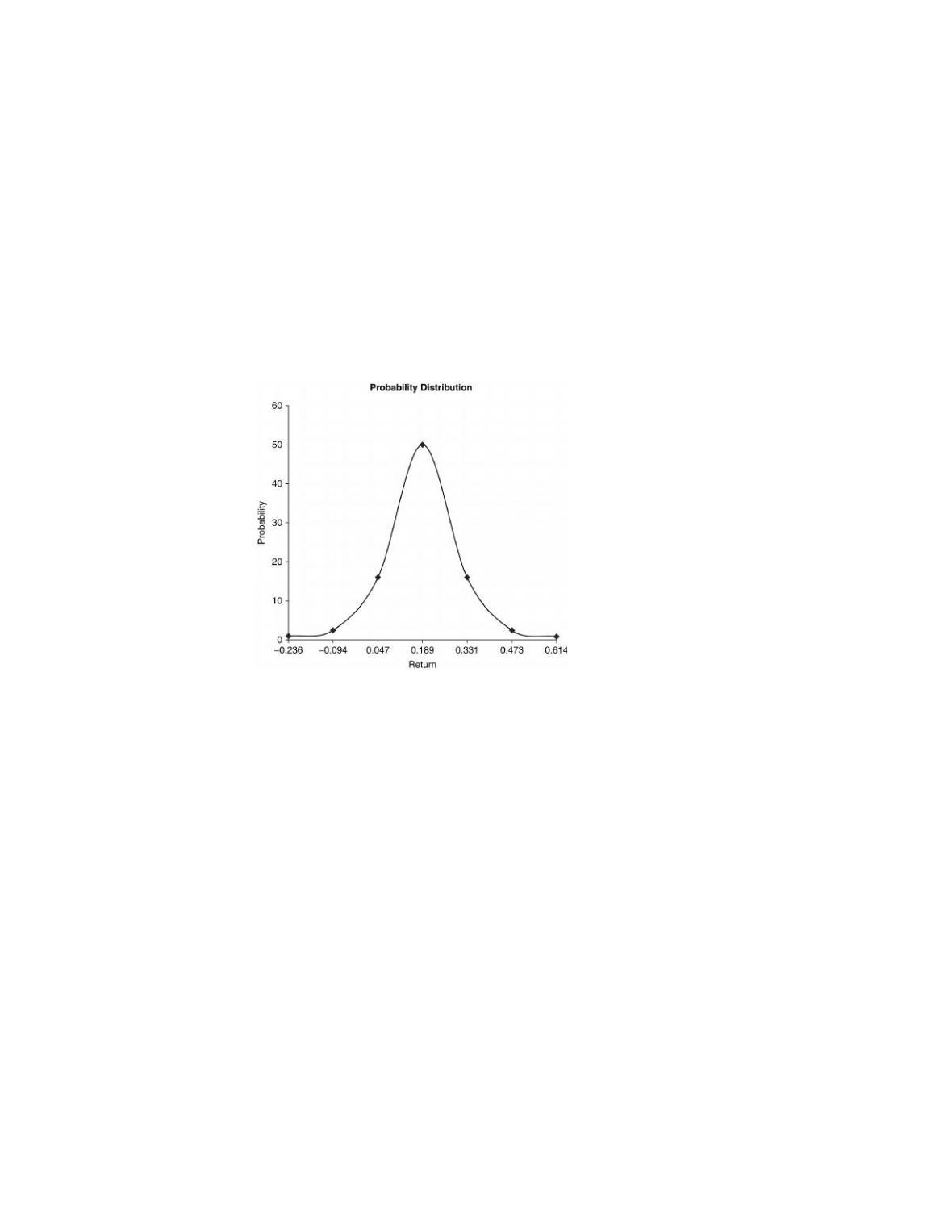
P8-12 Normal probability distribution (LG 2; Challenge)
a. Coefficient of variation: CV = σ , where so σ is the standard deviation of returns on the asset
and is the expected return. So, given the CV (0.75) and the expected return (0.189), solve for
standard deviation: 0.75
0.189 →
0.750.189 0.14175