Chapter 8 Risk and Return 161
Based on standard deviation, Asset G appears to have the greatest risk.
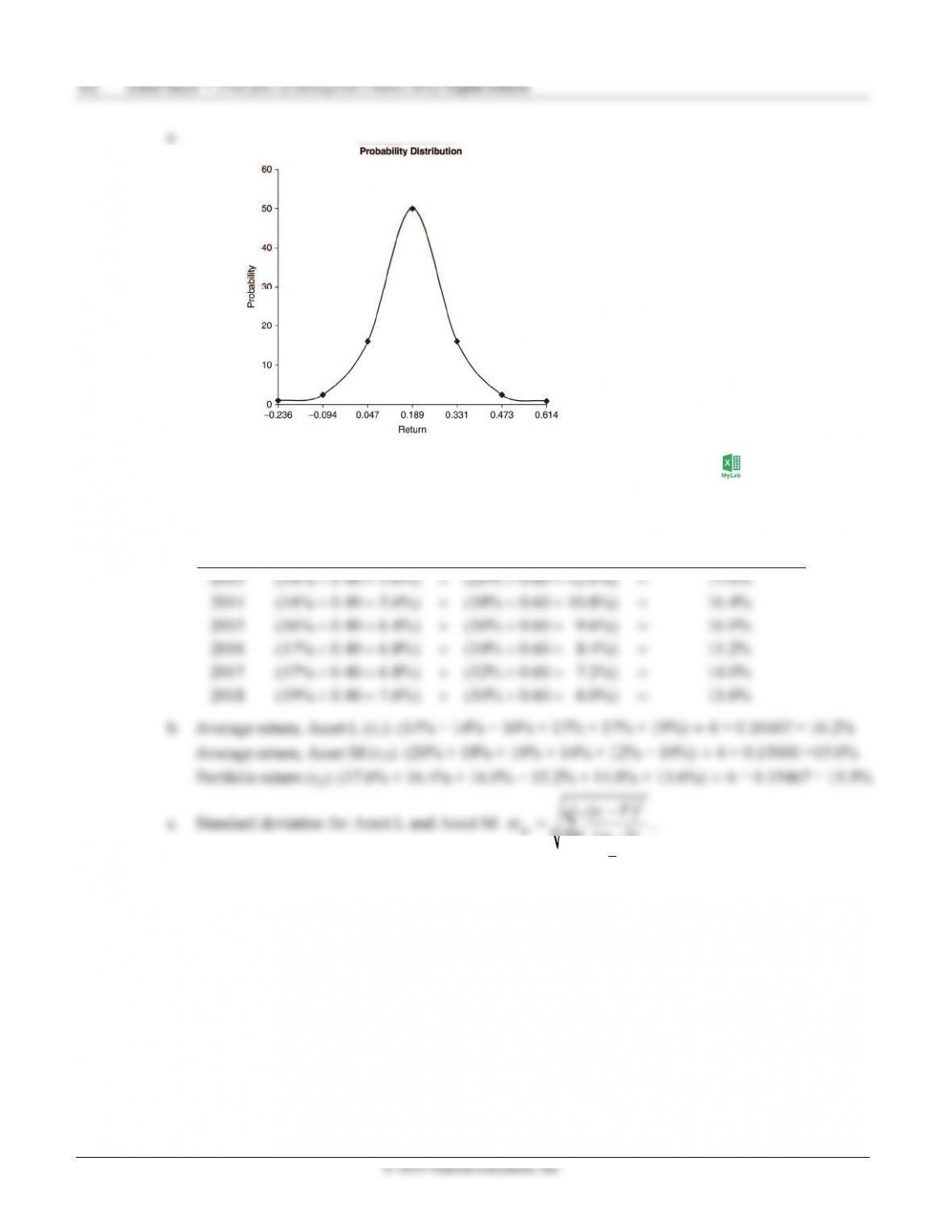
P8-12 Normal probability distribution (LG 2; Challenge)
a. Coefficient of variation: CV = σ ÷ r, where so σis the standard deviation of returns on the asset
(2) 95% of the outcomes will lie between ± 2 standard deviations of the expected value:
+2σ = 0.0189 + (2 × 0.14175) = 0.4725 –2σ = 0.0189 – (2 × 0.14175) = –0.0945
(3) 99% of the outcomes will lie between ±3 standard deviations of the expected value:
Asset H
Column →(1) (2) (3) (4) (5) (6)
Return
(r
i
)
Average
Return (r)= (1) ─ (2) = (3)
2
Probability
(P
ri
)= (4) x (5)
0.40 0.10 0.300 0.0900 0.100 0.009000
0.10 0.10 0.000 0.0000 0.400 0.000000
-0.20 0.10 -0.300 0.0900 0.100 0.009000
= 14.83%
© 2019 Pearson Education, Inc.
P8-13 Personal finance: Portfolio return and standard deviation (LG 3; Challenge)
a. Actual portfolio return for each year: rp = (wL × rL) + (wM × rM), where w is the portfolio weight of
asset L or M, and r is the actual return in a given year on asset L or M.
Year Asset L (wL × rL)
+
Asset M (wM
× rM) Portfolio Return (rp)
+
=
=
+
=
=
+
=
=
+
=
=
+
=
=
+
=
=
1
(1)
i
n
=
where ri is the asset return in year i (running to year n), and r is average return over n years:
164 Zutter/Smart • Principles of Managerial Finance Brief, Eighth Edition
© 2019 Pearson Education, Inc.
d and e.
The standard deviation (risk) of portfolio returns is 1.51%, lower than either asset (1.94% for
Asset L and 3.74% for Asset M). So holding the two assets as a portfolio yields a diversification
benefit, indicating the returns on Asset L and M must be less than perfectly positively correlated.
[Note: The actual correlation coefficient between the returns on Asset L and Asset M is
-0.9635—the assets are highly negatively correlated—but negative correlation is not necessary
for a diversification benefit.]
P8-14 Portfolio analysis (LG 3; Challenge)
a. Expected portfolio return:
Alternative 1: 100% Asset F
16.5% 16.5% 16.5% 16.5% 16.5%
4
p
r
+
++
==
Alternative 3: 50% Asset F + 50% Asset H
15.0% 16.0% 17.0% 18.0% 16.5%
4
p
r
+
++
==
1
(1)
i
n
=
where ri is asset return in year i (running to year n), and r is average return over n years:
+
Chapter 8 Risk and Return 165
© 2019 Pearson Education, Inc.
Alternative 1:
17.5%
F
16.5%
FG
16.5%
FH
= 1.291%
166 Zutter/Smart • Principles of Managerial Finance Brief, Eighth Edition
d. Summary:
r
σ
r CV
P8-15 Correlation, risk, and return (LG 4; Intermediate)
(2) Standard deviation of the portfolio will range from 5% (standard deviation of Asset V) and
10% (standard deviation of Asset W), depending on the weights of the assets in the portfolio.
(2) Students do not have enough information to determine the precise minimum standard
deviation obtainable through diversification, but it certainly exceeds 0% (because that is only
(2) Standard deviation of the portfolio will range from 0% (standard deviation if assets are
P8-16 Personal finance: International investment returns (LG 1 and LG 4; Intermediate)
a. Return Pesos = (24.75 – 20.5) ÷ 20.5 = 0.20732 = 20.73%
b. Purchase price Beginning of Year = Price in pesos ÷ Pesos per dollar = $2.22584 × 1,000 = $2,225.84
© 2019 Pearson Education, Inc.
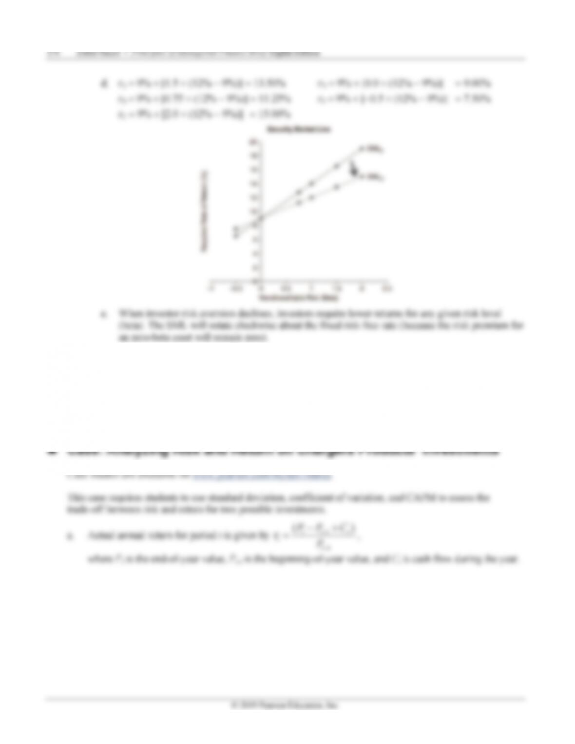
P8-19 Graphic derivation of beta (LG 5; Intermediate)
a. The returns for Biotech are more disperse, so it has a higher standard deviation.
P8-20 Interpreting beta (LG 5; Basic)
The impact of a change in market return for an asset with a beta of 1.20 if market return rises by:
P8-21 Betas (LG 5; Basic)
B 1.60 ×0.10 = 0.16 B 1.60 ×
−0.10 =−0.16
C −0.20 ×0.10 = −0.02 C −0.20 ×
−0.10 = 0.02
D 0.90 ×0.10 = 0.09 D 0.90 ×
−0.10 = −0.09
c. Asset B should be chosen because it will have the highest increase in return.
Chapter 8 Risk and Return 171
© 2019 Pearson Education, Inc.
−
+
Security analysts typically use statistical techniques to estimate an asset’s beta by obtaining a line
of best fit through historical asset and market returns. The slope of this line is beta. Data points—
that is, actual returns on the asset and market for a given period—will be randomly scattered
around the line no matter how well it “fits” the data. The point here is asset betas are estimates.
The CAPM return is, in a sense, a forecast and even good forecasts are subject to random error.
Another possibility is beta does not fully capture all nondiversifiable or systemic factors that
affect expected returns. Still another possibility is the firm behind the asset has changed, so the
beta estimated with historical data does not reflect the asset’s current beta.
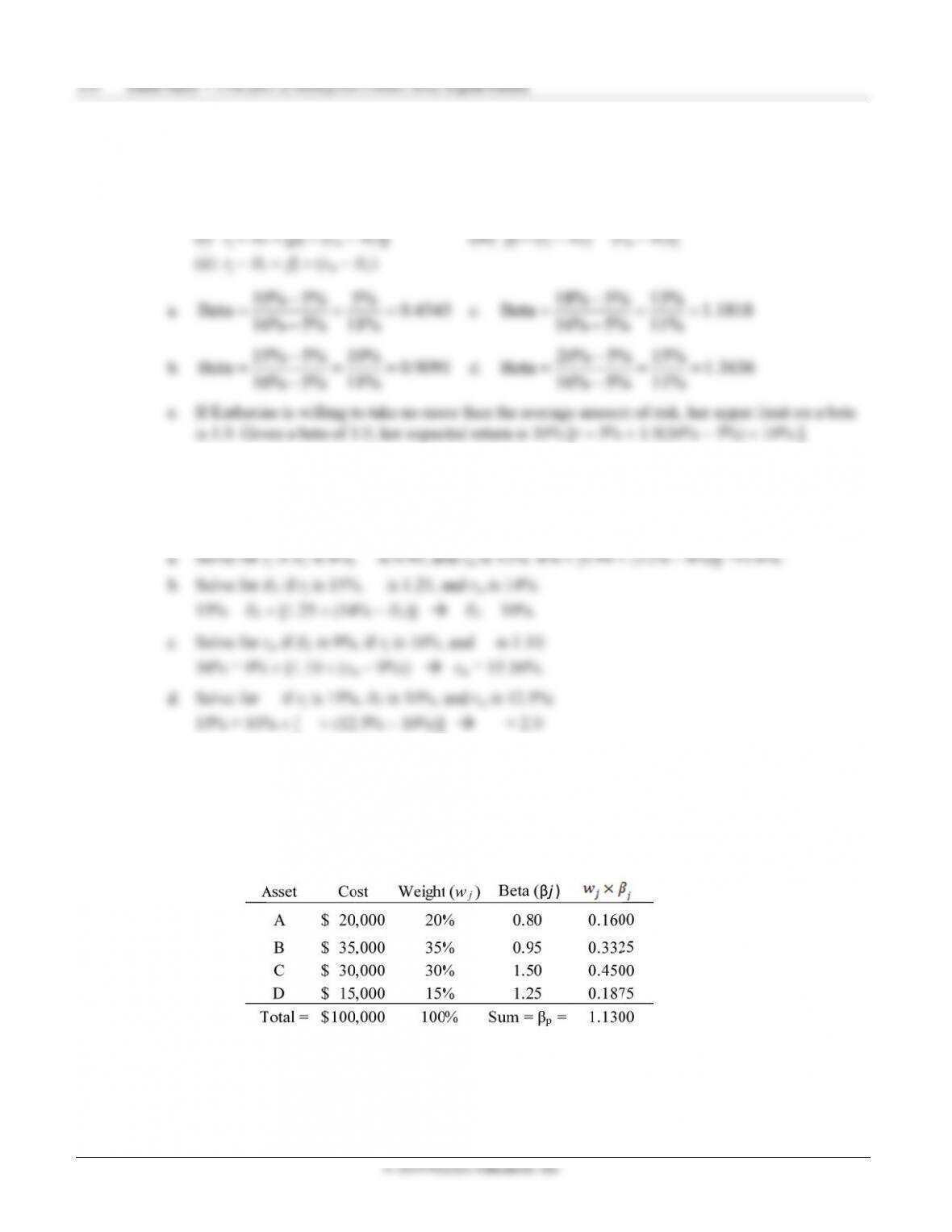
Asset
Actual
Return
CAPM
Return
Over- or
Underperformed
CAPM
A 8.00% 8.80% Under
B 6.86% 9.70% Under
D 12.50% 11.50% Over
© 2019 Pearson Education, Inc.
P8-30 Integrative: Risk, return, and CAPM (LG 6; Challenge)
a. Using the CAPM equation, rj = RF + [𝛽 × (rm − RF)], where RF is the risk-free rate, 𝛽 the project
beta , and rm the return on the market portfolio, solve for rj is the required return on each project j:
Project RF
+
[𝜷
𝒋
×
(rm
−
RF)] rj
+
−
=
+
−
=
+
−
=
+
−
=
+
−
−
=
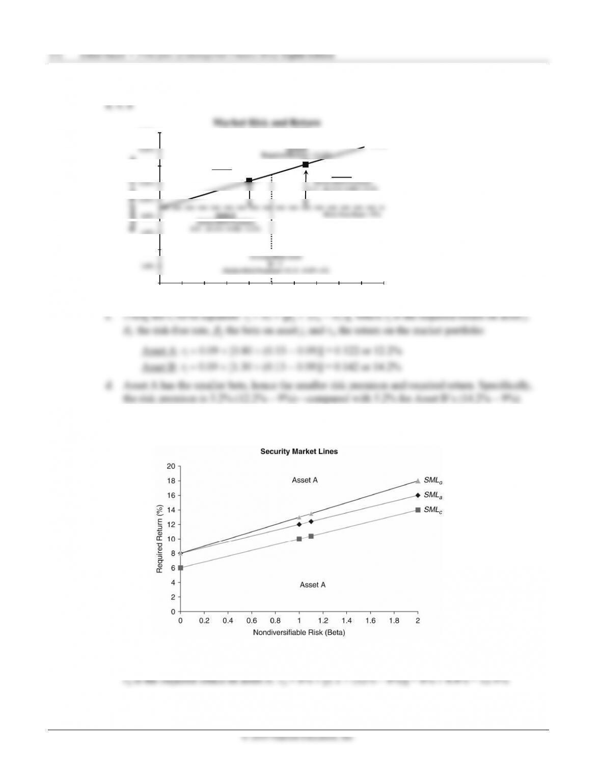
returns with the market return—yields the risk premium for the project’s nondiversifiable risk.
Projects A and C have more nondiversifiable risk than the market because their betas exceed 1.0;
they require risk premiums above the average risk premium. Projects B, D, and E have less
nondiversifiable risk than the market because their betas are less than 1.0; they carry risk
premiums below the average risk premium). Projects D and E are particularly noteworthy. Project
© 2019 Pearson Education, Inc.
P8-31 Ethics problem (LG 1; Intermediate)
Investors expect managers to take risks with their money, so it is not unethical for managers to make
risky investments with other people’s money. Managers do, however, have a duty to communicate
truthfully with investors about the risk they take. Portfolio managers should not take risks they do not
expect to generate returns sufficient to compensate investors for systemic risk.
© 2019 Pearson Education, Inc.
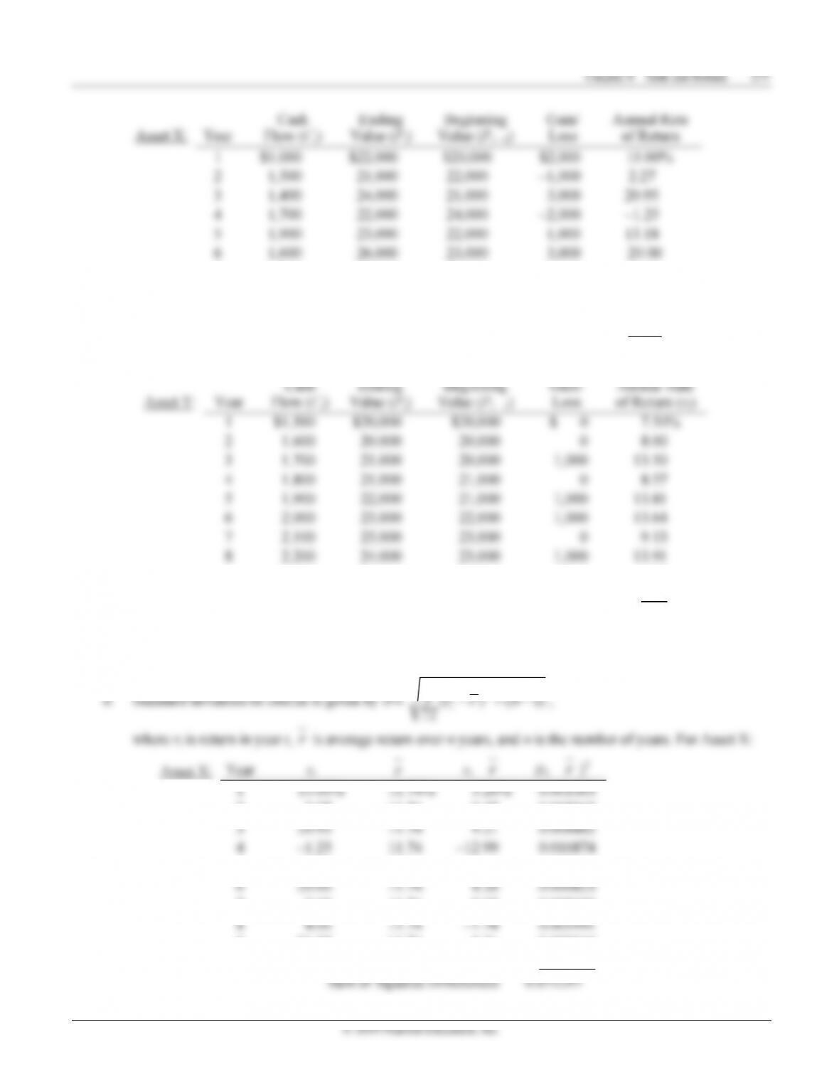
−
7 1,700 25,000 26,000
−
1,000 2.69
8 2,000 24,000 25,000
−
1,000 4.00
9 2,100 27,000 24,000 3,000 21.25
10 2,200 30,000 27,000 3,000 19.26
Ten-Year Average = 11.74%
Cash
Ending
Beginning
Gain
/
Annual Rate
9 2,300 25,000 24,000 1,000 13.75
10 2,400 25,000 25,000 0 9.60
Ten-Year Average = 11.14%
Mr. Sayou anticipates expected annual return over the next ten years will match average return over the
past 10 years, so expected return on Asset X is 11.74%, and expected return on Asset Y is 11.14%.
n
2 2.27 11.74
−
9.47 0.008968
−
5 13.18 11.74 1.44 0.000207
7 2.69 11.74 -9.05 0.008190
−
9 21.25 11.74 9.51
0.009044
10 19.26 11.74 7.52
0.005655
/
−

© 2019 Pearson Education, Inc.
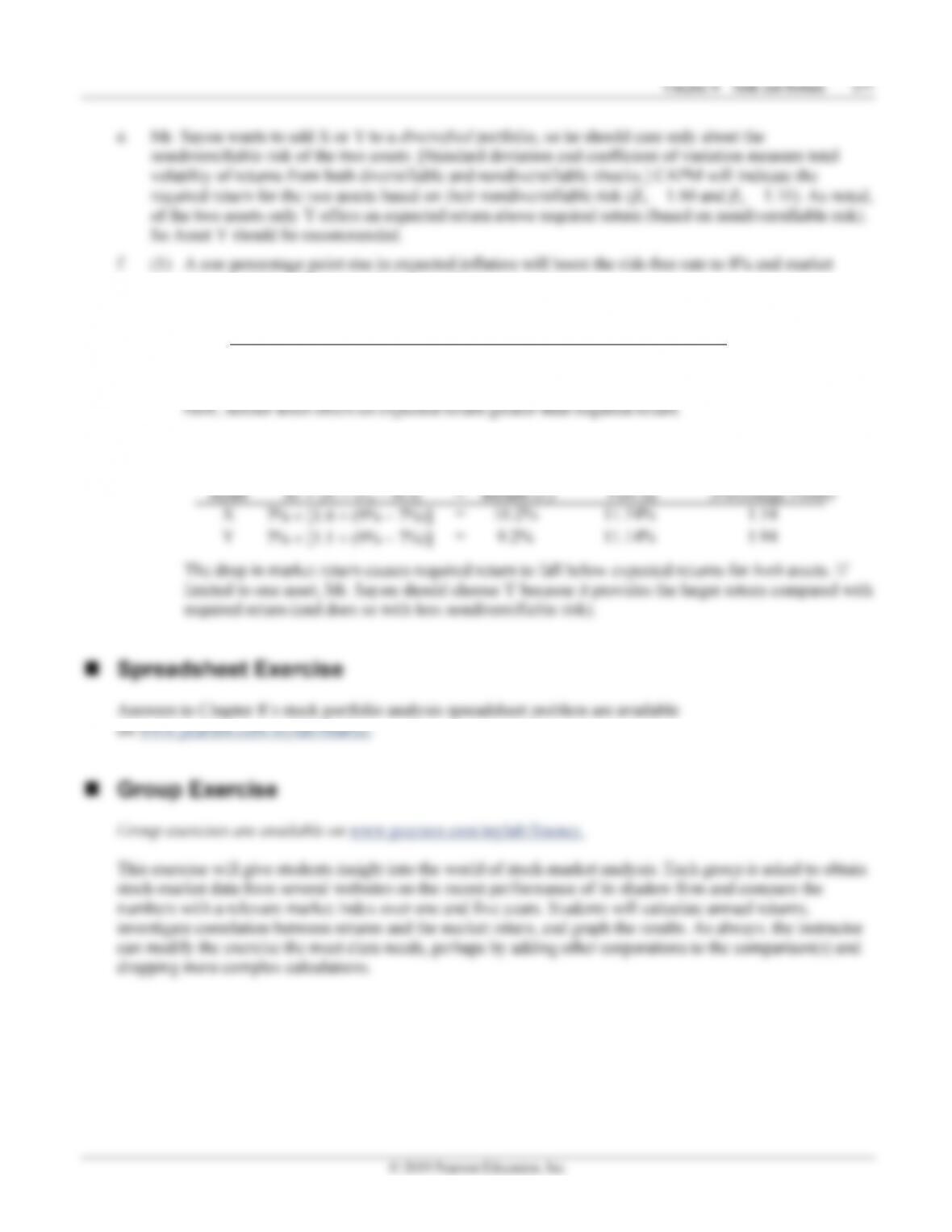
return to 11% and have the following effect on rx and ry:
Asset
CAPM:
RF + [bj
× (rm − RF)] =
Required
Return (rj)
Expected Return
Part (a)
X 8% + [1.6 × (11%
−
8%)] = 12.8% 11.74%
Y 8% + [1.1 × (11%
−
8%)] =11.3% 11.14%
(2) If investors become less risk averse, causing market return to fall to 9%, rx and ry will change to:
CAPM
Required
Expected Return
Difference
−
−