F
B U S I N E S S A N A L Y T I C S M O D U L E
Simulation
DISCUSSION QUESTIONS
1. The seven steps of simulation are define the problem;
introduce the important variables associated with the problem;
2. Advantages of simulation:
1. It is relatively straightforward and flexible.
2. It can be used to analyze large and complex real-world
situations that cannot be solved by conventional operations
4. It allows “time compression.”
6. It does not interfere with the real-world system.
7. It allows us to study interactive effects of individual
3. Disadvantages of simulation:
4. Simulated average demand is based on the simulation model
demand, and is a precise and unchanging value, the weighted aver–
age or expectation of the values of the variable being modeled.
LO F.2: Perform the five steps in a Monte Carlo simulation
AACSB: Reflective thinking
5. The role of random numbers in simulation is to help generate
should be very similar.
LO F.2: Perform the five steps in a Monte Carlo simulation
AACSB: Reflective thinking
7. Monte Carlo simulation is a technique that uses random
◼ Step 1: Establish a probability distribution for each random
random variable
◼ Step 3: Establish an interval of random numbers for each
AACSB: Application of knowledge
generation of simulation packages.
10. Special-purpose languages have these advantages:
(1) They require less programming time for large simulations.
346 BUSINESS ANALYTICS MODULE F SI M U LA T I O N
(3) They have random number generators already built-in as
subroutines.
LO F.4: Use Excel spreadsheets to create a simulation
AACSB: Information technology
11. The results would change, and perhaps significantly, if a
3
8:09
8
8:14
8:22
5
4
8:15
6
8:22
8:28
7
12. A computer is necessary for three reasons:
◼ It can perform the individual trials in much less time than
Day
Demand
Unsold
Profit
1
0
2
0
3
0
4
4
5
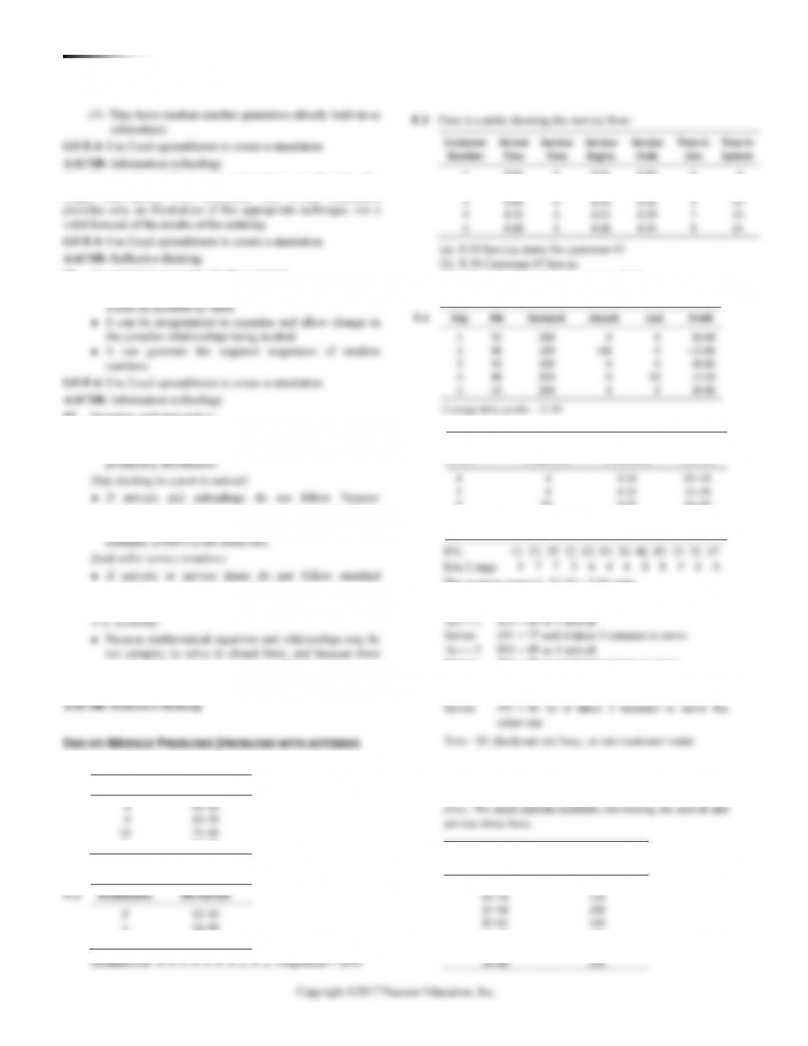
(c) 4.2 min average time in queue (= 21/5)
(d) 10.8 min average time in system (= 54/5)
F.3
Here is a table showing the service flow:
Customer
Arrival
Service
Service
Service
Time in
Time in
Number
Time
Time
Begins
Ends
Line
System
1
8:01
6
8:01
8:07
0
6
2
8:06
7
8:07
8:14
1
8
6
7
Copyright ©2017 Pearson Education, Inc.
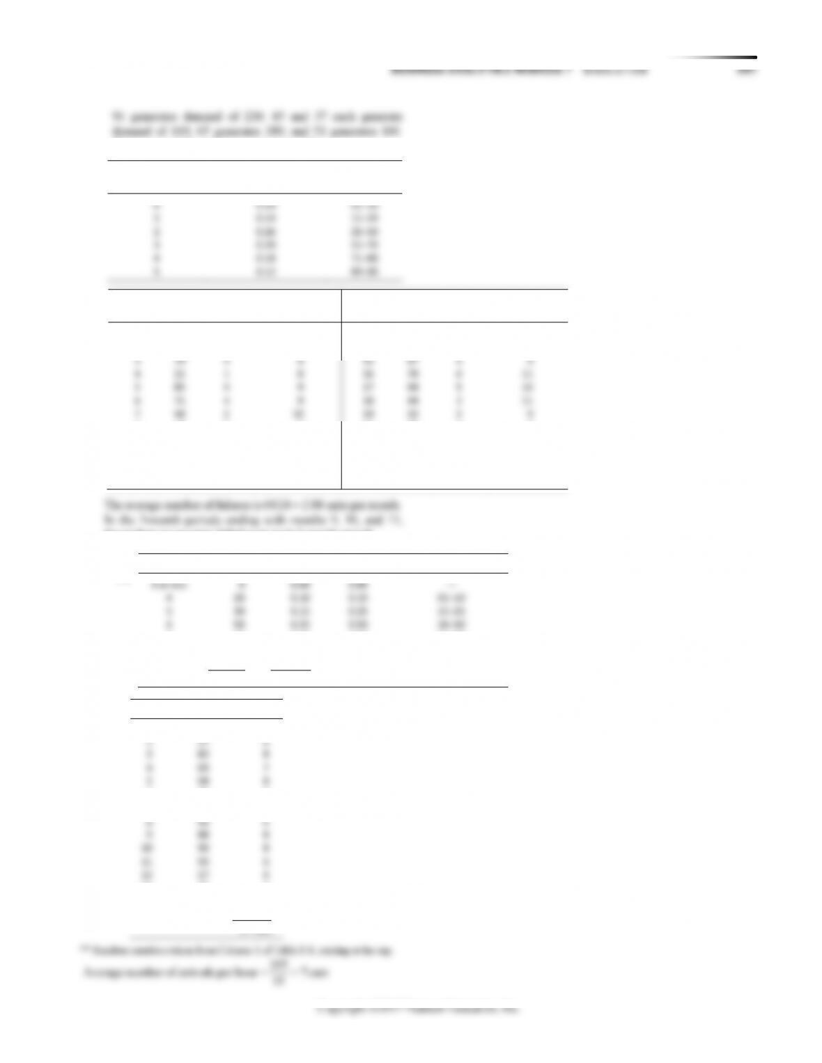
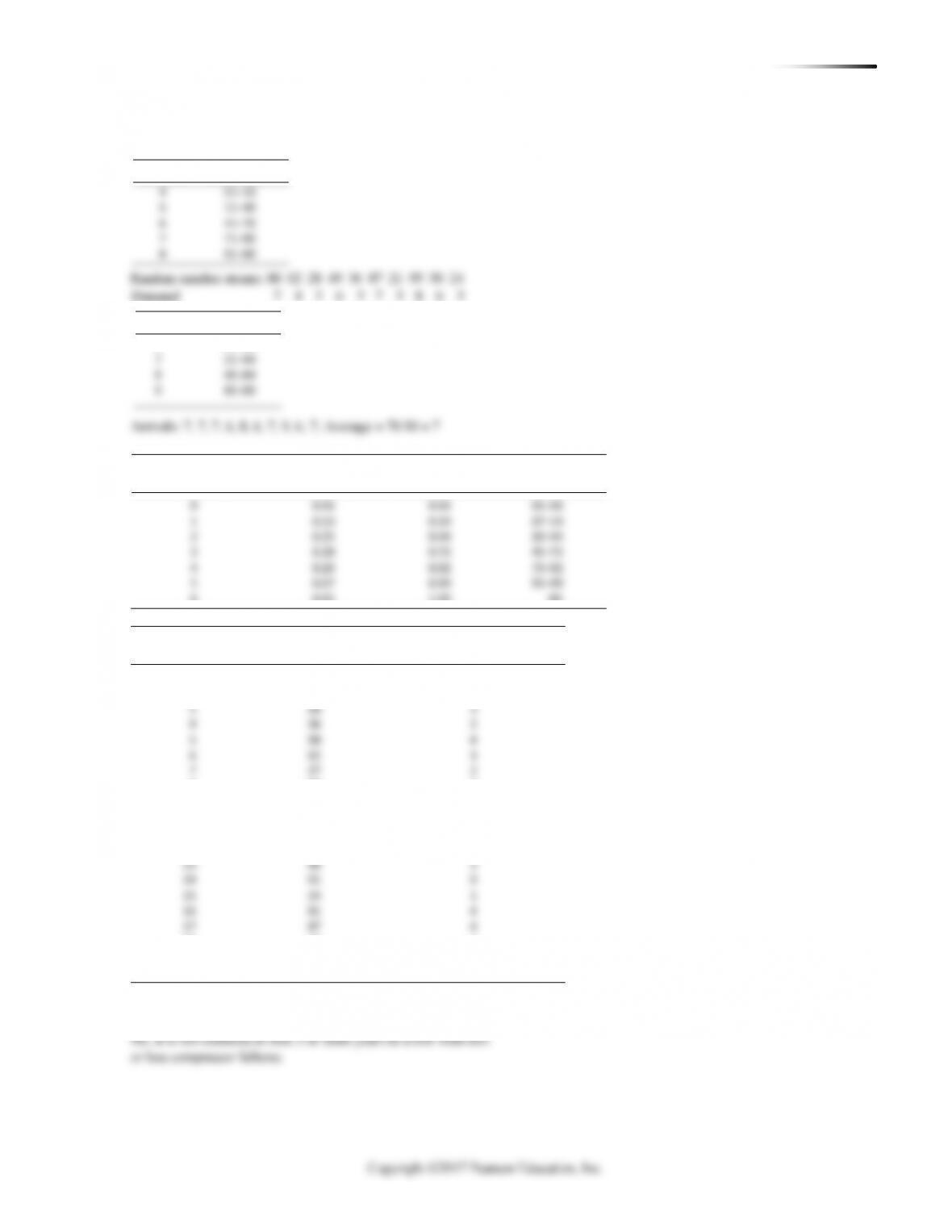
Their sum is 840, and their average is 168.
F.8
Number of Failed
Boxes per Month
Probability
RN Intervals
3
79
4
9
15
97
5
9
4
21
1
8
16
4
11
5
85
4
9
17
94
5
14
6
71
4
9
18
44
2
11
fewer than seven units failed over each 3-month stretch.
4
20
0.10
0.10
01–10
5
30
0.15
0.25
11–25
(c)
Hour
Random**
Arrivals
1
52
7
2
37
6
3
82
8
4
69
7
5
98
8
6
96
8
7
33
6
8
50
6
9
88
8
10
90
8
11
50
6
12
27
6
13
45
6
14
81
8
15
66
7
15
7
48
2
19
32
2
9
No. of
3-Month
No. of
3-Month
Month
RN
Failures
Total
Month
RN
Failures
Total
1
37
2
13
41
2
7
2
60
3
14
31
2
8
8
39
2
8
20
85
4
8
9
31
2
6
21
64
3
9
10
35
2
6
22
84
4
11
11
12
1
5
23
63
3
10
12
73
4
7
24
29
2
9
F.9
(a)
(b)
Number
Freq.
Probability
Cumulative
Random No. Interval
3 or less
0
0.00
0.00
—
6
50
0.25
0.50
26–50
7
60
0.30
0.80
51–80
8
40
0.20
1.00
81–00
9 or more
0
—
—
—
= 200
= 1.00
348 BUSINESS ANALYTICS MODULE F SI M U LA T I O N
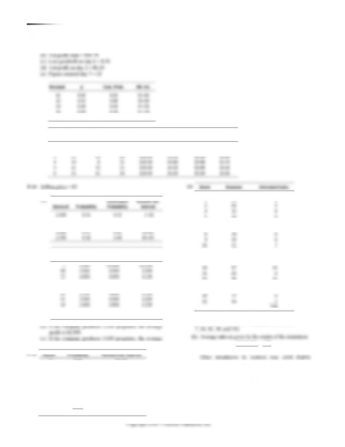
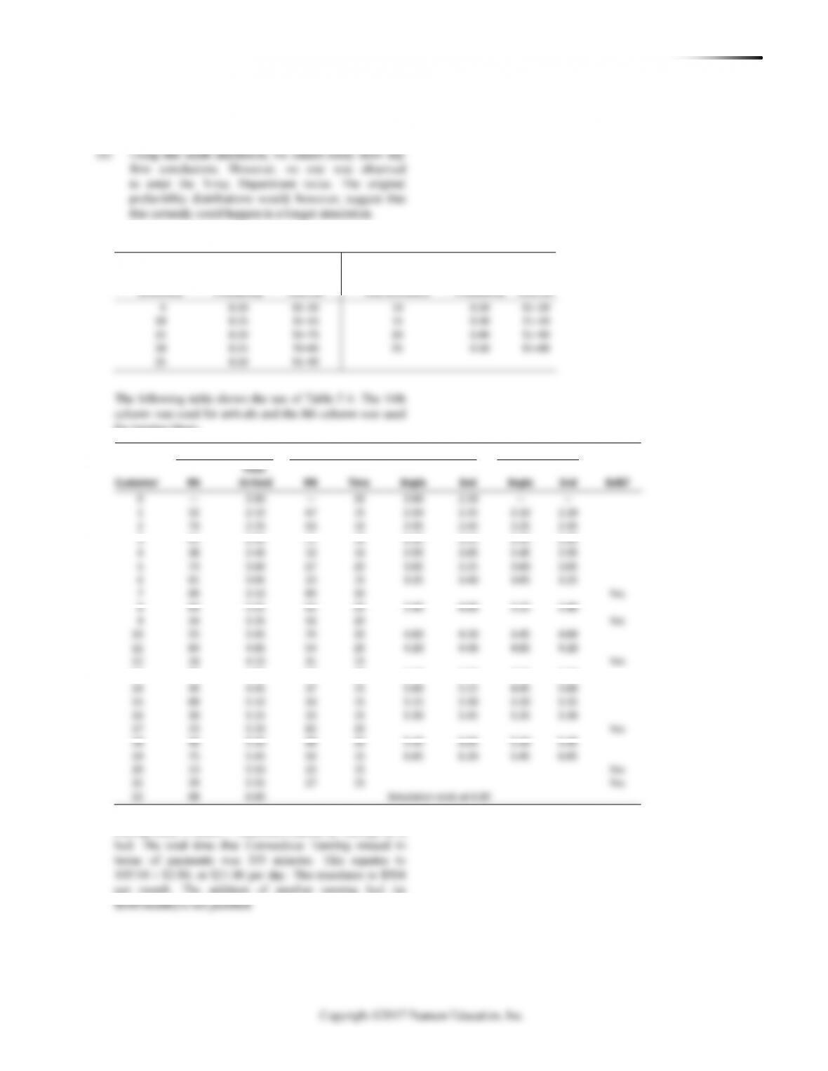
F.10 (a) Day 3 demand = 24
RN. Int.
3,000
3,120
Heater
Week
3
21
52
24
$10.50
$4.20
$0.30
$6.00
4
24
21
$10.50
$4.80
$0.00
$5.70
5
21
22
21
$10.50
$4.20
$0.00
$6.30
25
0.30
1.00
71–00
Papers
Random
Goodwill
Day
Ordered
Number
Demand
Revenue
Cost
Cost
Net Profit
1
22
37
22
$11.00
$4.40
$0.00
$6.60
2
22
19
21
$10.50
$4.40
$0.00
$6.10
BUSINESS ANALYTICS MODULE F SI MU L A TI O N 349
A simulation that lasts for longer than 20 time periods will result
in answers that are even closer.
F.13*
Demand
RN Interval
Demand: 7 4 5 6 5 7 5 8 6 5
7
21–44
8
45–84
3
68
3
4
36
2
5
90
4
6
62
3
7
27
2
13
46
3
14
01
0
15
14
1
16
81
4
17
87
4
F.14*
#Cars
RN Interval
6
01–20
F.15*
Number of Air
Relative Frequency
Cumulative
Random Number
Conditioner Failures
(Probability)
Probability
Interval
6
0.01
1.00
00
Number of A/C Compressors
Simulated Period
Random Number**
to Fail This Year
1
50
3
2
28
2
8
50
3
9
18
1
10
36
2
11
61
3
12
21
2
18
72
3
19
80
4
20
46
3
** Random numbers taken from Column 3 of Table F.4, starting at
the top.
350 BUSINESS ANALYTICS MODULE F SI M U LA T I O N
1
2
3
4
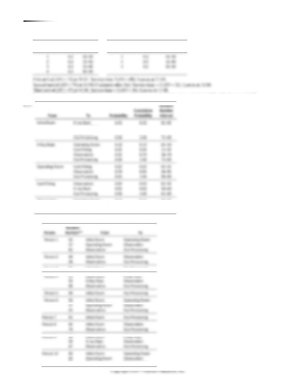
Number**
Person 1
52
Initial Exam
Operating Room
37
Operating Room
Observation
82
Observation
Out-Processing
Person 2
69
Initial Exam
Observation
98
Observation
Out-Processing
Person 3
96
Initial Exam
Out-Processing
Person 4
33
Initial Exam
X-Ray Dept.
50
X-Ray Dept.
Observation
88
Observation
Person 5
90
Initial Exam
Out-Processing
Person 6
50
Initial Exam
Operating Room
27
Operating Room
Observation
45
Observation
Out-Processing
Person 7
81
Initial Exam
Out-Processing
Person 8
66
Initial Exam
Observation
74
Observation
Out-Processing
Person 9
30
Initial Exam
X-Ray Dept.
Observation
0.10
0.70
61–70
Out-Processing
0.30
1.00
71–00
X-Ray Dept.
Operating Room
0.10
0.10
01–10
Cast-Fitting
0.25
0.35
11–35
Observation
0.35
0.70
36–70
Out-Processing
0.30
1.00
71–00
Operating Room
Cast-Fitting
0.25
0.25
01–25
Observation
0.70
0.95
26–95
Out-Processing
0.05
1.00
96–00
Cast-Fitting
Observation
0.55
0.55
01–55
X-ray Dept.
0.05
56–60
Out-Processing
0.40
1.00
61–00
Initial Exam
X-ray Dept.
0.45
0.45
01–45
Operating Room
0.15
0.60
46–60
Observation
Operating Room
0.15
0.15
01–15
X-ray Dept.
0.15
0.30
16–30
Out-Processing
0.70
1.00
31–00
F.16
Time Between
Arrivals
Prob.
RN Interval
Service Time
Prob.
RN Interval
Fourth arrival (RN = 03) at 11:07. Must wait 1 minute for service to start. Service time = 1 minute (RN = 24). Leaves at 11:09.
(a)
Simulation
80
Observation
Out-Processing
BUSINESS ANALYTICS MODULE F SI MU L A TI O N 351
** Random number taken from Column 1 of Table F.4.
Reading top-to-bottom.
for tanning times.
Arrived
Simulation ends at 6:00
F.18
The Monte Carlo simulation tables are:
Time between
Arrivals
RN
Time in Tanning
RN
(minutes)
Probability
Interval
Bed (minutes)
Probability
Interval
Arrivals
Tanning Time
Wait Time
Time