B
B U S I N E S S A N A L Y T I C S M O D U L E
Linear Programming
DISCUSSION QUESTIONS
1. Students may select from eight LP applications given in the
introduction: school bus scheduling, police patrol allocation,
objective function and constraints
2. LP theory states that the optimum lies on a corner. All three
solution techniques make use of the “corner point” feature.
3. The feasible region is the area bounded by the set of problem
4. Each LP problem that has been formulated correctly does
in which the optimal solution lies on a constraint that is parallel to
AACSB: Reflective thinking
5. The objective function contains the profit or cost information
LO B.1: Formulate linear programming models, including an
6. Before activity values can be placed into the objective, they
LO B.1: Formulate linear programming models, including an
7. As long as the costs do not change, the diet problem always
provides the same answer. In other words, the diet is the same
every day. Unlike animals, people enjoy variety, and variety can-
8. The number of feasible solutions is infinite. We only need to
point to determine the optimal solution.
9. Shadow price or dual: the value of one additional unit of a
resource, such as one more hour of a scarce labor resource or one
corner point.
point, whereas the iso-profit line method draws a series of parallel
method
LO B.3: Graphically solve an LP problem with the corner-point
12. When two constraints do not cross at an axis, we use simul-
LO B.2: Graphically solve an LP problem with the iso-profit line
13. (a) Adding a new constraint will reduce the size of the feasi-
BUSINESS ANALYTICS MODULE B LI N E A R PR O G R A M M I N G 293
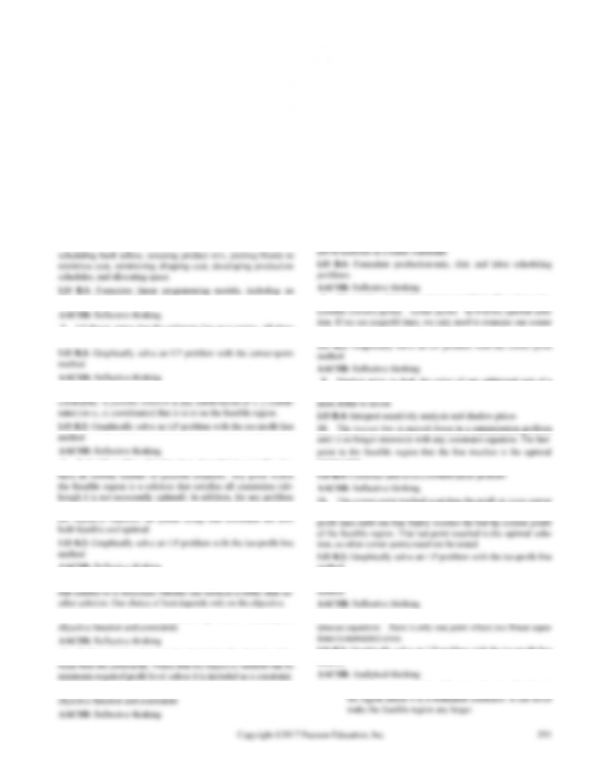
Let x1 = number of air conditioners to be produced
2x1 + 1x2 140 (drilling)
x1, x2 0 (non-negativity)
Profit:
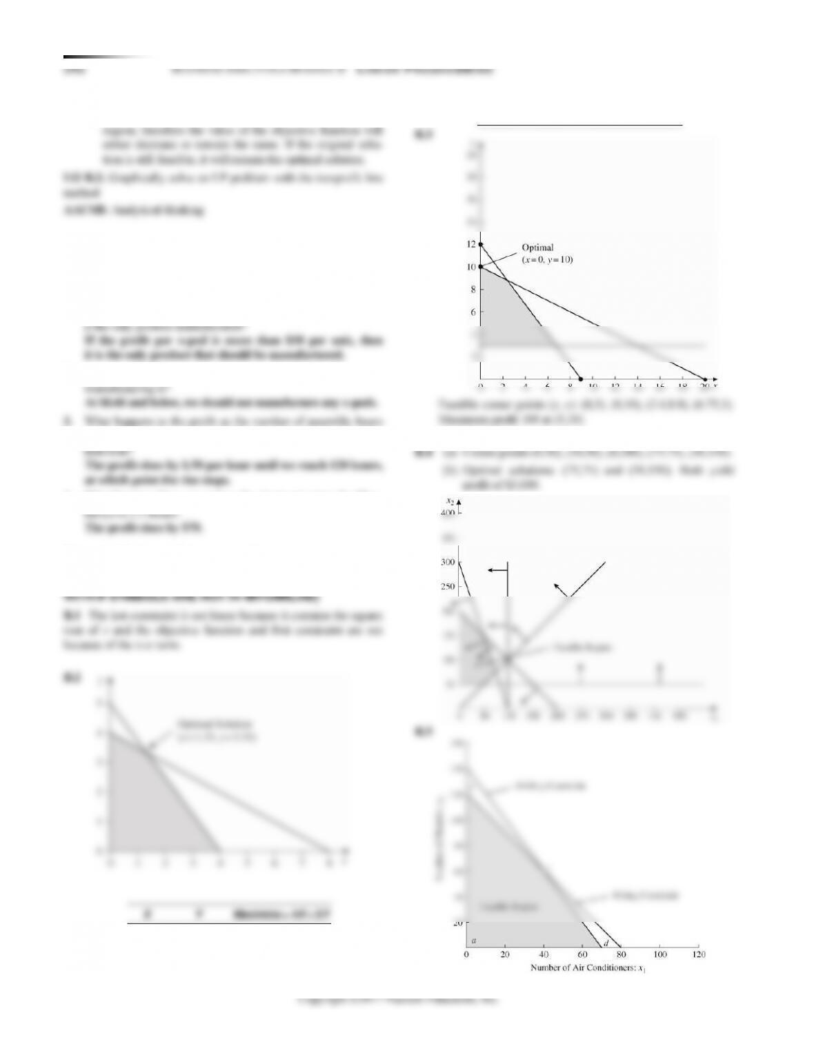
B.6
20x1 + 30x2 6,000 (zinc)
= $17,714.10
@c: (x1 = 200, x2 = 0) Obj = 90 200 + 70 0
= $18,000.00*
* The optimal solution is to produce 200 Model A gates, and 0
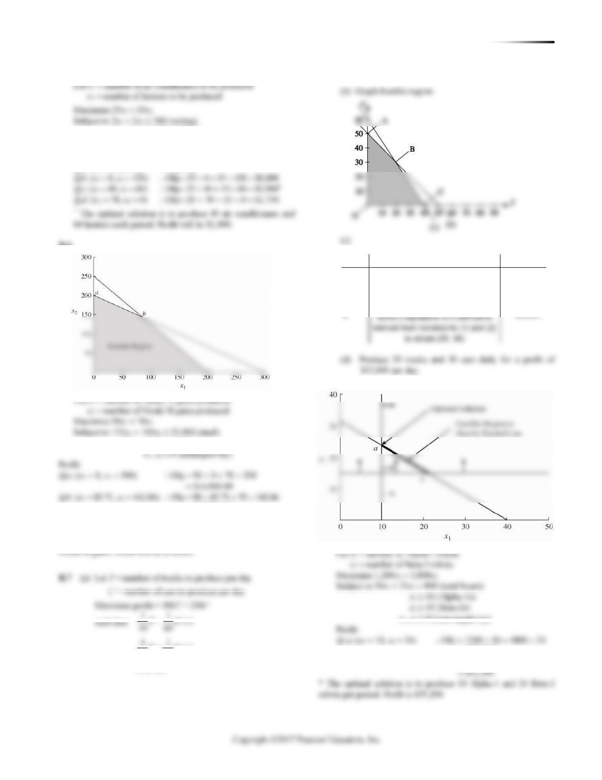
B.8
= $55,200*
@ b: (x1 = 21.25, x2 = 15) Obj = 1200 21.25 + 1800 15
+1
50 50
, 0
TC
TC
Point
Coordinates
Profit
O
(0, 0)
0
A
(0, 50)
11,000
C
(40 ,0)
12,000
BUSINESS ANALYTICS MODULE B LI N E A R PR O G R A M M I N G 295
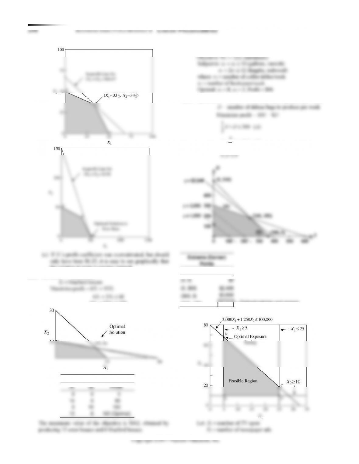
Maximize exposures = 35,000X1 + 20,000X2
B.15* Let x = number of standard model to produce
*
12
12
@ : ( 262.5, 25) Obj 9 262.5 20 25 $2,862.50
@ : ( 300, 0) Obj 9 300 20 0 $2,700.00
b x x
c x x
= = = + =
= = = + =
B.20*
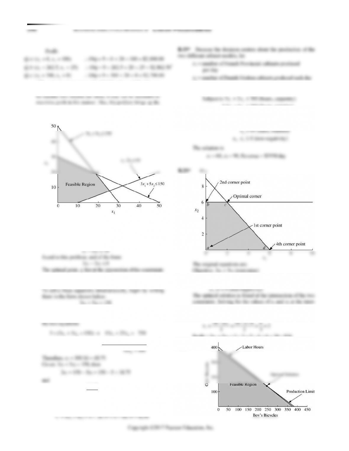
3x1 + 5x2 150
5x1 + 3x2 150
5x1 + 3x2 = 150
Multiply the first equation by 5, the second by −3, and add
x1 = number of French Provincial cabinets produced
per day
x2 = number of Danish Modern cabinets produced each day
The equations become:
Objective: 28x1 + 25x2 (maximize revenue)
12
12
12
1
2
12
Subject to 3 2 360 (hours, carpentry)
1.5 1 200 (hours, painting)
0.75 0.75 125 (hours, finishing)
60 (units, contract)
60 (units, contract)
, 0 (non-negativity)
xx
xx
xx
x
x
xx
+
+
+
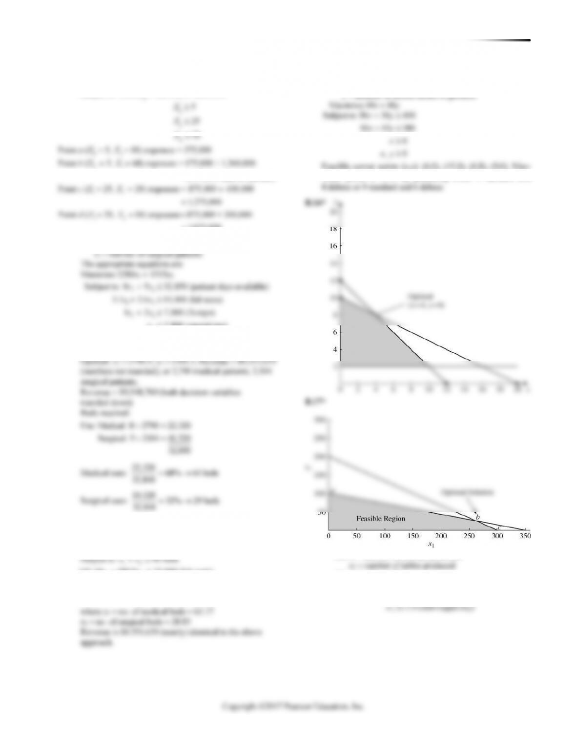
Subject to x2 6
3x1 + 2x2 18
section, we have:
x2 = 6
* The optimal solution is to make 262.5 benches and 25 tables per
period. Profit will be $2,862.50. Because benches and tables may
be matched (two benches per table), it may not be reasonable to
maximize profit in this manner. Also, this problem brings up the
proper interpretation of the statement “One should make 262.5
(a fractional quantity) benches per period.”
B.18*
BUSINESS ANALYTICS MODULE B LI N E A R PR O G R A M M I N G 297
Maximize: 57x1 + 55x2
Subject to: x1 + x2 390
B.22 (a) Using POM for Windows software, we find that the
optimal solution is:
B.23 (a) VA1 fertilizer shipped to Customer A from Warehouse W1
B.24* (a) Maximize 18.79x1 + 6.31x2 + 8.19x3 + 45.88x4 + 63x5
+ 4.1x6 + 81.15x7 + 50.06x8 + 12.79x9
const 5: 10.9x1 + 2x2 + 2.3x3 + 4.9x5 + 10x6 + 11.1x7
+ 12.4x8 + 5.2x9 + 6.1x10 + 7.7x11 + 5x12
const 15: 1x9 50
(c)
Description
Variables and Coeffi-
cients?
What Type?
RHS?
298 BUSINESS ANALYTICS MODULE B LI N E A R PR O G R A M M I N G
Solution Value = 9683.229
Shadow
Slack or
Original
Lower
Upper
Prices
Surplus
RHS
Limit
Limit
const 1
2.711812
0.00
980.00
861.5504
1,024.236
const 2
0.00
113.866
400.00
286.1337
Infinity
const 3
10.6486
0.00
600.00
587.7851
608.5712
const 4
2.182708
0.00
2,500.00
1,889.72
2,534.683
const 5
0.00
258.885
1,800.00
1,541.115
Infinity
const 6
0.00
8.52954
1,000.00
991.4705
Infinity
const 7
0.00
0.00
0.00
const 8
−46.1866
0.00
20.00
17.91737
41.84552
const 9
−26.4548
0.00
10.00
const 10
0.00
10.00
16.993
const 11
0.00
0.00
const 12
−27.37
0.00
20.00
16.50255
37.096
const 13
−34.041
10.00
10.00
12.01538
const 14
−32.6758
0.00
20.00
17.09391
23.00434
const 15
−11.75
0.00
50.00
39.20661
116.4478
const 16
−10.8416
0.00
20.00
14.30611
79.923
const 17
0.00
20.00
15.88757
68.822
const 18
0.00
10.00
const 19
−29.243
0.00
20.00
15.45261
22.44298
const 20
0.00
2.20215
10.00
−Infinity
12.20215
const 21
−48.87
0.00
10.00
8.355577
12.84913
(b) The shadow prices are given in the table above.
(d) Two tons of steel at a total cost of $8,000 implies a cost per
limit is 1,024 pounds.
(e) Change coefficient for variable x14 in objective function
x3
10.00
0.00
8.19
−Infinity
32.86478
x4
16.993
0.00
45.88
38.60427
60.25521
x5
7.056
0.00
63.00
42.61333
71.26741
x6
20.00
0.00
4.10
−Infinity
30.43315
x7
10.00
0.00
81.15
−Infinity
106.3944
x8
20.00
0.00
50.06
−Infinity
76.83481
x9
50.00
0.00
12.79
−Infinity
26.18145
x11
20.00
0.00
17.91
−Infinity
29.29111
x12
57.697
0.00
49.99
91.778
x13
20.00
0.00
24.00
−Infinity
45.986
x14
10.00
0.00
8.88
−Infinity
80.82936
Solution Value = 8865.5
Optimal
Reduced
Original
Lower
Upper
Value
Cost
Coefficient
Limit
Limit
x1
0.00
1.23911
18.79
−Infinity
20.02911
x2
20.00
0.00
6.31
−Infinity
51.68507
B.24* (cont.)
BUSINESS ANALYTICS MODULE B LI N E A R PR O G R A M M I N G 299
Solution Value = 8865.5
Shadow
Slack or
Original
Lower
Upper
Prices
Surplus
RHS
Limit
Limit
const 1
2.74856
0.00
980.00
913.6641
993.1374
const 2
0.00
113.879
400.00
286.1211
Infinity
const 3
9.197201
0.00
600.00
587.7851
601.577
const 4
2.343288
0.00
2,500.00
2,342.00
2,512.443
const 5
0.00
266.934
1,800.00
1,533.066
Infinity
const 6
0.00
2.36523
1,000.00
997.6348
Infinity
const 7
0.00
0.00
0.00
−Infinity
0.00
const 8
−45.3751
0.00
20.00
19.45971
41.84552
const 9
−24.6748
0.00
10.00
8.988791
19.9601
const 10
0.00
6.993
10.00
−Infinity
16.993
const 11
0.00
7.05643
0.00
−Infinity
7.056433
const 12
−26.3331
0.00
20.00
19.15507
37.096
const 13
−25.2444
0.00
10.00
9.459686
12.01538
const 14
−26.7748
0.00
20.00
19.5257
23.00434
const 15
−13.3914
0.00
50.00
39.20661
62.76064
const 16
−12.6447
0.00
20.00
17.28464
31.80706
const 17
−11.3811
0.00
20.00
18.28127
32.64
const 18
0.00
47.70
10.00
−Infinity
57.69793
const 19
−21.986
0.00
20.00
19.46232
22.44298
const 20
71.9494
0.00
10.00
9.155032
12.20215
const 21
−42.6476
0.00
10.00
9.67822
12.84913
B.24* (cont.)
(f) Constraints 7 through 11 become: x1 0, x2 0, x3 0,
x4 0, x5 0. The following results:
Solution Value = 9380.23
Optimal
Reduced
Original
Lower
Upper
Value
Cost
Coefficient
Limit
Limit
x1
0.00
7.90441
18.79
−Infinity
26.69441
x2
0.00
16.81
6.31
−Infinity
23.1219
x3
0.00
10.9491
8.19
−Infinity
19.1391
x4
0.00
2.75734
45.88
−Infinity
48.63734
x5
28.72255
0.00
63.00
61.75618
63.859
x6
20.00
0.00
4.10
−Infinity
12.95034
x7
10.00
0.00
81.15
−Infinity
86.86531
x8
37.51722
0.00
50.06
49.69948
71.07961
x9
50.00
0.00
12.79
−Infinity
23.18852
x10
20.00
0.00
15.88
−Infinity
20.73238
x11
33.94098
0.00
17.91
17.22904
18.570
x12
37.485
0.00
49.99
48.67592
51.016
x13
20.00
0.00
24.00
−Infinity
24.49456
x14
10.00
0.00
8.88
−Infinity
70.86956
x15
10.27741
0.00
77.01
75.18908
77.47366