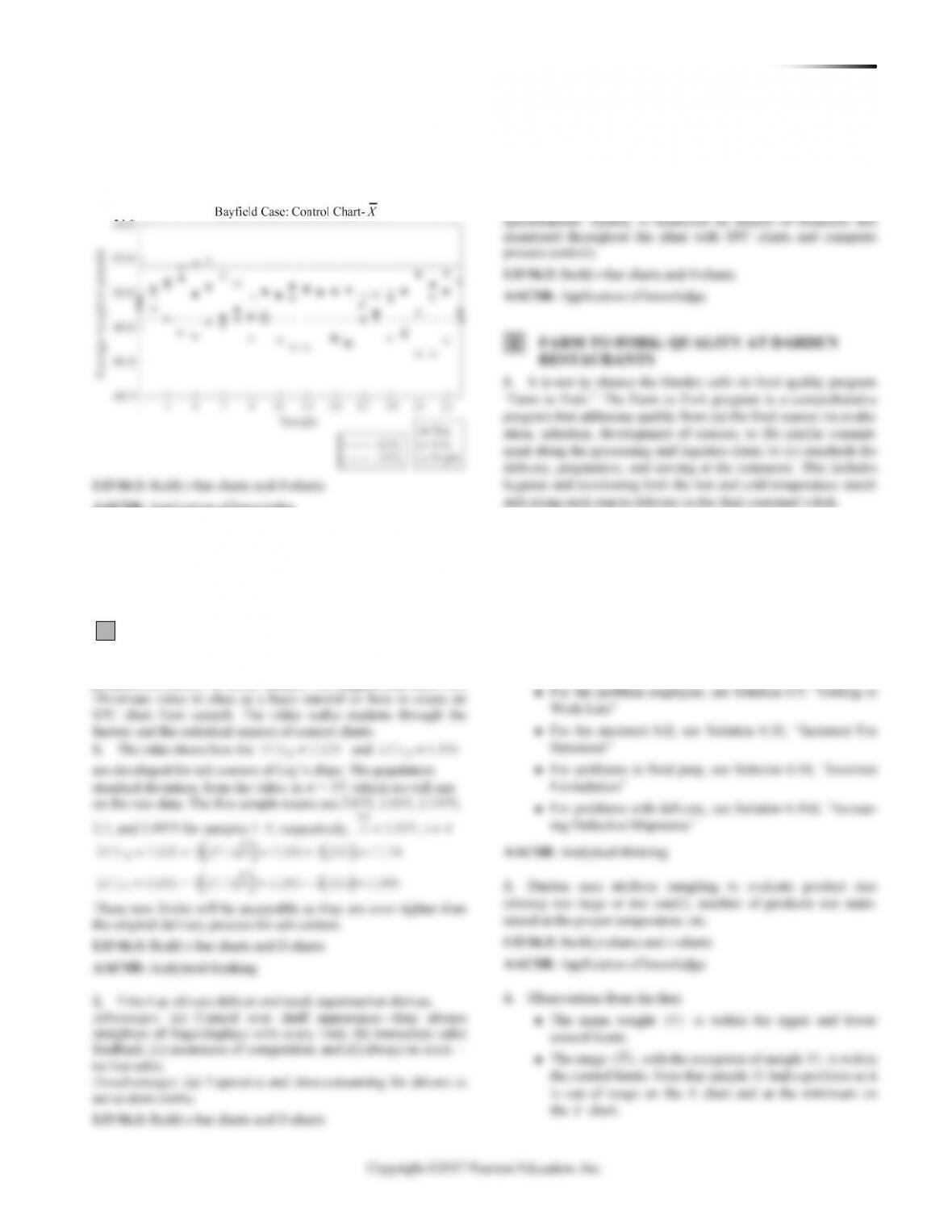
6
S U P P L E M E N T
Statistical Process Control
DISCUSSION QUESTIONS
1. Shewhart’s two types of variation, common and special
causes, are also called natural and assignable variation.
LO S6.1: Explain the purpose of a control chart
LO S6.1: Explain the purpose of a control chart
AACSB: Application of knowledge
5. The 5 steps are:
1. Collect 20 to 25 samples, often of n = 4 or 5 each;
compute the mean and range of each sample.
2. Compute the overall means (
x
and
R
), set appropriate
control limits using the new data.
LO S6.4: List the five steps involved in building control charts
6. Text list includes machine wear, misadjusted equipment,
LO S6.1: Explain the purpose of a control chart
AACSB: Application of knowledge
7. Two sigma covers only 95.5% of all natural variation; even in
the absence of assignable cause, points will fall outside the control
size. The control charts presented here should not be used if the
sample size varies.
LO S6.1: Explain the purpose of a control chart
11. Cpk, the process capability index, is one way to express
process capability. It measures the proportion of natural variation
(3) between the center of the process and the nearest specifica-
tion limit.
AACSB: Application of knowledge
14. A run test is used to help spot abnormalities in a control
chart process. It is used if points are not individually out of con-
88 SUPPLEMENT 6 ST AT I ST I CA L PR OC ES S CO N TR O L
15. Managerial issues include:
◼ Selecting places in a process that need SPC
◼ Deciding which type of control charts best fit
◼ Setting rules for workers to follow if certain points or pat-
terns emerge
LO S6.3: Build x-bar charts and R-charts
estimate the quality of a lot.
LO S6.7: Explain acceptance sampling
18. The two risks when acceptance sampling is used are type I
error: rejecting a good lot; type II error: accepting a bad lot.
LO S6.7: Explain acceptance sampling
19. A process that has a capability index of one or greater—a
“capable” process—produces small percentages of unacceptable
items. The capability formula is built around an assumption of
2. If we use a two-sigma control chart, what are the UCL and
LCL? Is the process more out of control?
The control limits are tighter. UCL = 16.667 and LCL =
15.333. Now five points are out of control.
3. What happens if the Z-value increases?
Now the control limits are wider at Z = 4, only one point is
out of control.
3. Suppose that the sample size used was actually 120 instead of
the 100 that it was supposed to be. How does this affect the chart?
The overall percentage of defects drops and, in addition,
the UCL and LCL get closer to the center line and each other.
4. What happens to the chart as we reduce the Z-value?
The chart gets “tighter.” The UCL and LCL get closer to
the center line and each other.
2. Increase the standard deviation. At what value will the curve
cross the upper specification?
About .9
END–OF-SUPPLEMENT PROBLEMS (PROBLEMS WITH ASTER-
ISKS APPEAR IN MYOMLAB ONLY)
S6.1
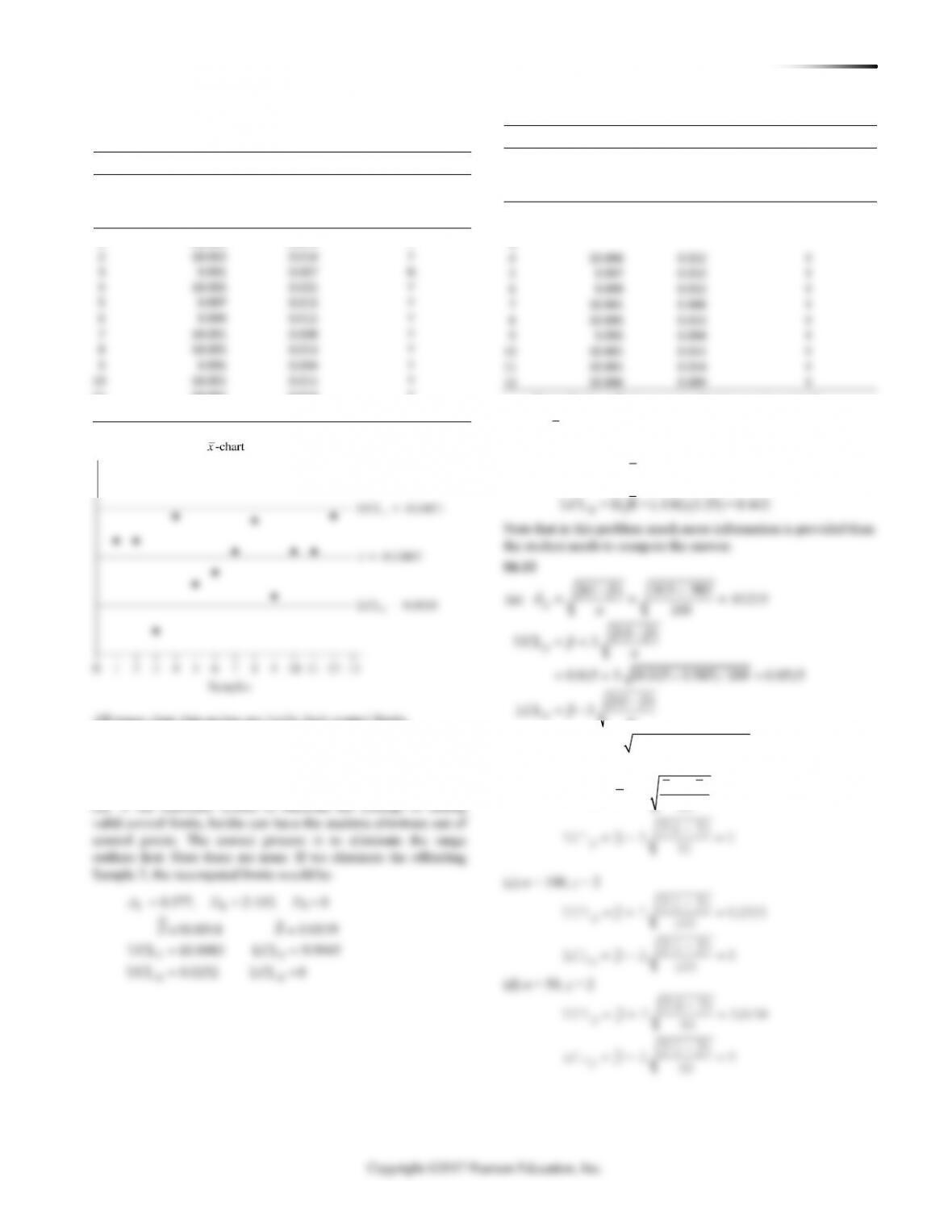
0.1 0.1 0.0167
6
36
xn
= = = =
( )
( )
= + = + =
= = =
1.72
UCL 50 2 50 2 .77 51.54
5
1.72
LCL 50 50 .77 48.46
5
x
x
– 2 – 2
The control limits are tighter, but the confidence level has dropped.
S6.3 The relevant constants are:
2 4 3
= 0.419 = 1.924 = 0.076A D D
25
SUPPLEMENT 6 ST AT ISTIC AL PROC ES S CO N T R O L 89
( )
( )
(b) LCL 3 420 3 5 405
UCL 3 420 3 5 435
X
X
xn
xn
= − = − =
= + = + =
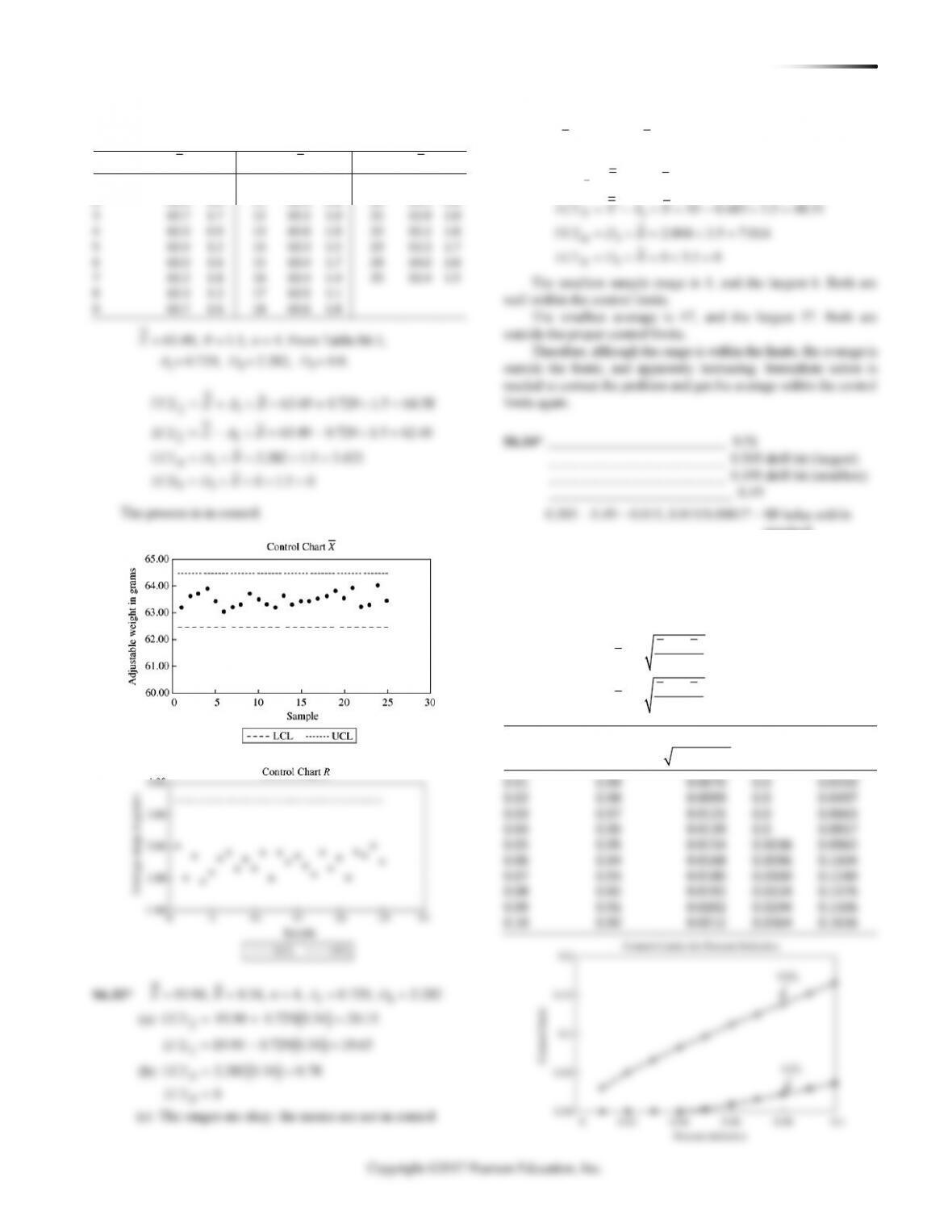
S6.5 From Table S6.1, A2 = 0.308, D4 = 1.777, D3 = 0.223
= +
2
UCL
xx A R
2
LCL
xx A R= −
S6.6
2
2
4
3
UCL 2.982 0.729 1.024 3.728
LCL 2.982 0.729 1.024 2.236
UCL 2.282 1.024 2.336
LCL 0 1.024 0
X
X
R
R
X A R
X A R
DR
DR
= + = + =
= − = − =
= = =
= = =
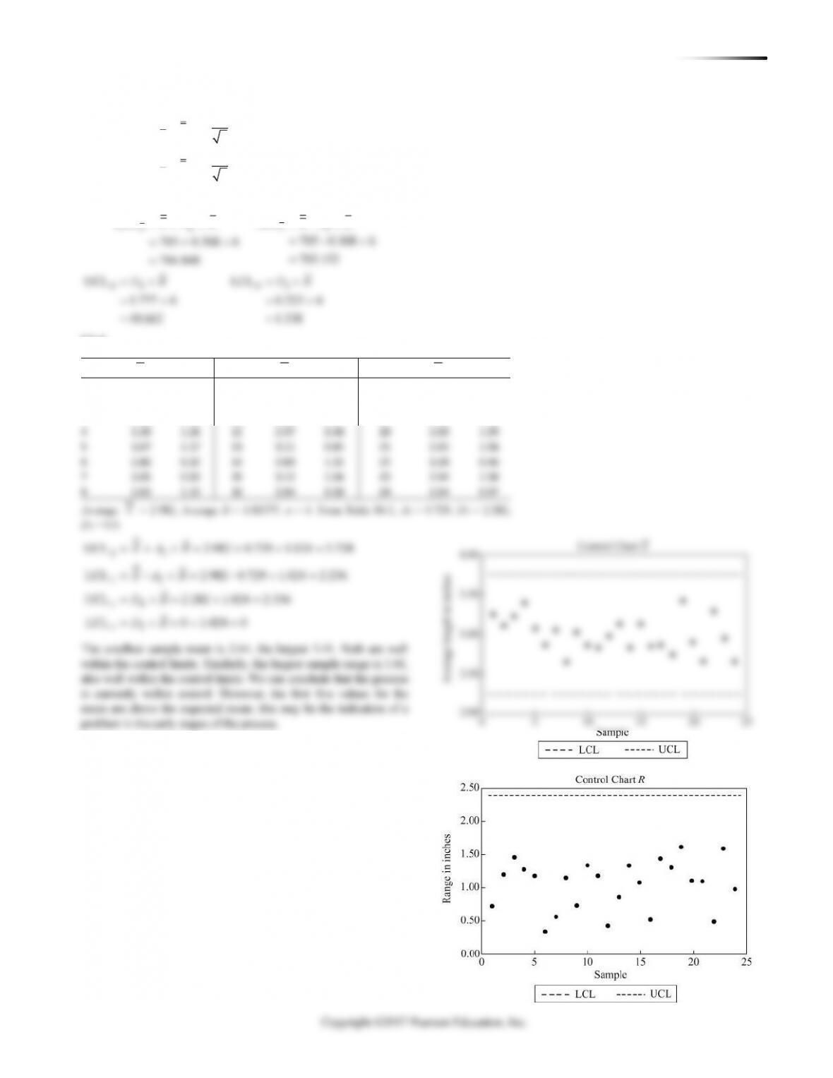
The smallest sample mean is 2.64, the largest 3.41. Both are well
within the control limits. Similarly, the largest sample range is 1.61,
also well within the control limits. We can conclude that the process
is currently within control. However, the first five values for the
mean are above the expected mean; this may be the indication of a
problem in the early stages of the process.
4
3.39
1.26
12
2.97
0.40
20
2.89
1.09
5
3.07
1.17
13
3.11
0.85
21
2.65
1.08
6
2.86
0.32
14
2.83
1.31
22
3.28
0.46
7
3.05
0.53
15
3.12
1.06
23
2.94
1.58
8
2.65
1.13
16
0.50
24
2.64
0.97
Hour
X
R
Hour
X
R
Hour
X
R
1
3.25
0.71
9
3.02
0.71
17
2.86
1.43
2
3.10
1.18
10
2.85
1.33
18
2.74
1.29
3
3.22
1.43
11
2.83
1.17
19
3.41
1.61
90 SUPPLEMENT 6 ST AT I ST I CA L PR OC ES S CO N TR O L
S6.7
Sample 1
6.025
0.4
(d) -chart:R
R4
R3
4.48 mm
UCL 1.777(4.48) 7.96 mm
LCL .223(4.48) 1.00 mm
R
DR
DR
=
= = =
= = =
(e) If the desired nominal line is 155 mm, then:
UCL 155 (.308 4.48) 155 1.38 156.38
LCL 155 (.308 4.48) 155 1.38 153.62
X
X
= + = + =
= − = − =
S6.8 (a)
(b) With z = 3,
0.12
U CL 16 3 16 .12 16.12
3
0.12
LCL 16 3 16 .12 15.88
3
X
X
= + = + =
= − = − =
UCL 1.141
LCL 0
R
R
=
=
S6.10
10, 3.3XR==
(a) Process (population) standard deviation () = 1.36,
(b) Using
x
( )
x
= + =
UCL 10 3 0.61 11.83
(d) Yes, both mean and range charts indicate process is
in control.
S6.11
= = =
==
==
==
2 4 3
(a) .577, 2.115, 0
10.0005 0.0115
UCL 10.0071 LCL 9.9939
UCL 0.0243 LCL 0
xx
RR
A D D
XR
Sample 2
6.05
0.4
Sample 3
5.475
1.5
Sample 4
6.075
0.3
Sample 5
6.625
0.4
156.9 153.2 153.6 155.5 156.6
(a) 155.16 mm
5
4.2 4.6 4.1 5.0 4.5
(b) 4.48 mm
5
X
R
+ + + +
==
+ + + +
==
Standard deviation of the sampling means
1.36 5
0.61
x
=
=
=
=
=
UCL and LCL
384
xZ xx
n
x
SUPPLEMENT 6 ST AT ISTIC AL PROC ES S CO N T R O L 91
(b)
Original Data
Are Both the Mean
Sample
and Range
Sample
Mean (in.)
Range (in.)
in Control?
1
10.002
0.011
Y
2
10.002
0.014
Y
3
9.991
0.007
N
4
10.006
0.022
Y
5
9.997
0.013
Y
6
9.999
0.012
Y
7
10.001
0.008
Y
8
10.005
0.013
Y
9
9.995
0.004
Y
10
10.001
0.011
Y
11
10.001
0.014
Y
12
10.006
0.009
Y
Revised Control Limits
Are both the Mean
Sample
and Range
Sample
Mean (in.)
Range (in.)
in Control?
1
10.002
0.011
Y
2
10.002
0.014
Y
3
4
10.006
0.022
Y
5
9.997
0.013
Y
6
9.999
0.012
Y
7
10.001
0.008
Y
8
10.005
0.013
Y
9
9.995
0.004
Y
10
10.001
0.011
Y
11
10.001
0.014
Y
12
10.006
0.009
Y
These limits reflect a process that is now in control.
S6.12
R= 3.25
mph, Z = 3,with n = 8, from Table S6.1, D4 =
1.864, D3 = .136
4
UCL = D R = (1.864)(3.25) = 6.058
LCL = D R = (.136) (3.25) = 0.442
R
92 SUPPLEMENT 6 ST AT I ST I CA L PR OC ES S CO N TR O L
(e) When the sample size increases,
( )
1
ˆ
p
pp
n
−
=
is smaller.
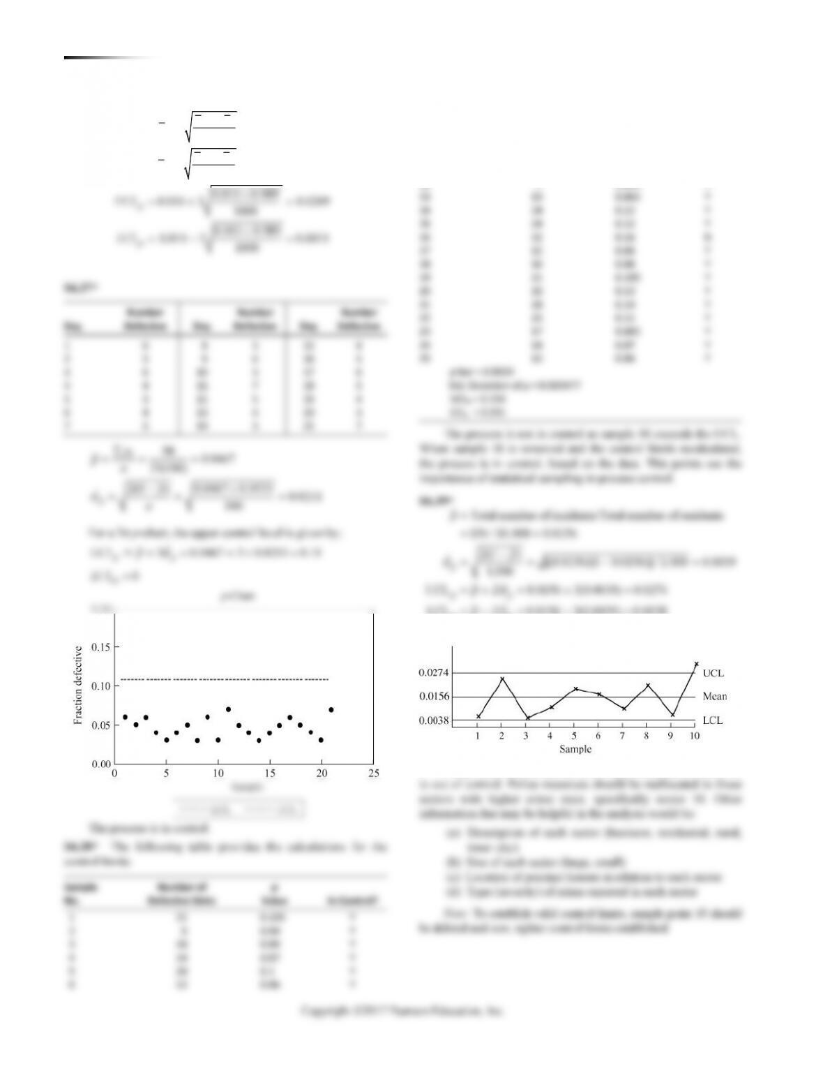
UCL 0.057 3(0.023) 0.057 0.069 0.126
LCL 0.057 3(0.023) 0.057 0.069 0.012 0
= + = + =
= − = − = − =
p
p
(b) The process is out of control on the third day (of the
next 3 days). For example, .13 exceeds the upper
control limit of 0.126.
()
()
1
UCL 3
1
LCL 3
0.015 0.985
UCL 0.015 3 0.0313
500
0.015 0.985
LCL 0.015 3 0.0013, or zero
p
p
p
pp
pn
pp
pn
S6.16 −
=+
−
=−
= + =
= − = −
(b) The LCL cannot be negative because the percent defective can
never be less than zero.
(c) The industry standards are not as strict as those at Birmingham
S6.20 (a) n = 200,
p
= 50/10(200) = 0.025
(1 )
UCL 3
(1 )
LCL 3
0.025 0.975
UCL 0.025 3 0.0581
200
0.025 0.975
LCL 0.025 3 0.0081, or zero
200
p
p
p
p
pp
pn
pp
pn
−
=+
−
=−
= + =
= − = −
SUPPLEMENT 6 ST AT ISTIC AL PROC ES S CO N T R O L 93
(b) Use mean of 6 weeks of observations
36 =6
6
for
,c
as true
c
is unknown.
(c) It is in control because all weeks’ calls fall within
interval of [0, 13].
(d) Instead of using we now use
LCL = 4 – 3(2) = –2, or 0
Week 4 (11 calls) exceeds UCL. Not in control.
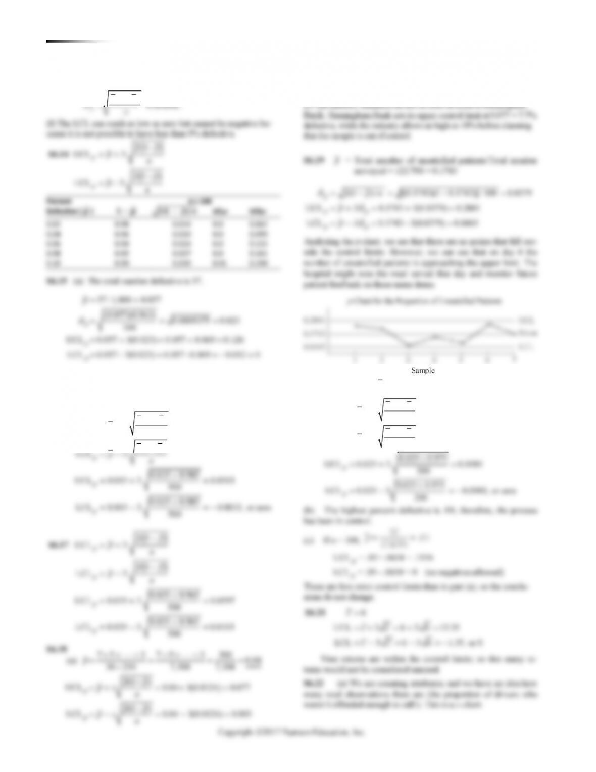
S6.23
213/5 42.6 test errors per school
UCL 3 42.6 3 42.6 42.6 19.5806 62.1806
LCL 3 42.6 – 3 42.6 42.6 19.5806 23.0194
c
c
c
cc
cc
==
= + = + = + =
= − = = − =
The chart indicates that there are no schools out of control. It
also shows that 3 of 5 schools fall close to or below the process
average, which is a good indication that the new math program has
been taught as effectively at one school in the county as another.
Whether or not the new math program is effective would require
comparisons of this year’s test results with results from previous
years (under the old program) or comparisons with national
per-formance data.
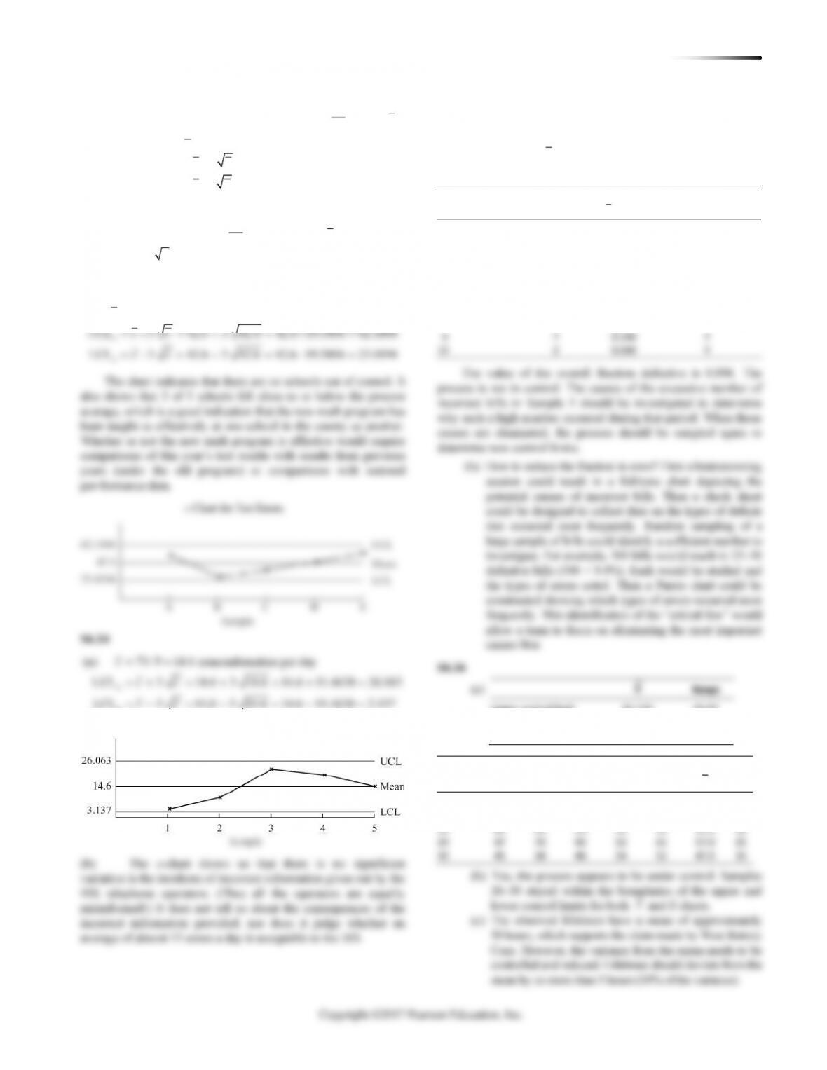
S6.24
(a) 73/ 5 14.6 nonconformities per day
UCL 3 14.6 3 14.6 14.6 11.4630 26.063
LCL 3 14.6 3 14.6 14.6 11.4630 3.137
c
c
c
cc
cc
==
= + = + = + =
= − = − = − =
(b) The c-chart shows us that there is no significant
variation in the incidents of incorrect information given out by the
IRS telephone operators. (Thus all the operators are equally
misinformed!) It does not tell us about the consequences of the
incorrect information provided, nor does it judge whether an
average of almost 15 errors a day is acceptable to the IRS.
S6.25
(a)
ˆ
0.094, 0.041
UCL 0.218 LCL 0
==
==
p
pp
p
No. of
Is the Billing
Sample No.
Incorrect Bills
p
Value
Process in Control?
1
6
0.120
Y
2
5
0.100
Y
3
11
0.220
N
4
4
0.080
Y
5
0
0.000
Y
6
5
0.100
Y
7
3
0.060
Y
8
4
0.080
Y
9
7
0.140
Y
10
2
0.040
Y
The value of the overall fraction defective is 0.094. The
process is not in control. The causes of the excessive number of
incorrect bills in Sample 3 should be investigated to determine
why such a high number occurred during that period. When those
causes are eliminated, the process should be sampled again to
determine new control limits.
(b) How to reduce the fraction in error? First a brainstorming
session could result in a fishbone chart depicting the
potential causes of incorrect bills. Then a check sheet
could be designed to collect data on the types of defects
that occurred most frequently. Random sampling of a
large sample of bills could identify a sufficient number to
investigate. For example, 300 bills would result in 25–30
defective bills (300 × 9.4%). Each would be studied and
the types of errors noted. Then a Pareto chart could be
constructed showing which types of errors occurred most
frequently. This identification of the “critical few” would
allow a team to focus on eliminating the most important
causes first.
S6.26
(a)
X
Range
Upper control limit
61.131
41.62
Center line (avg)
49.776
19.68
Lower control limit
38.421
0.00
Recent Data Sample
Hour
1
2
3
4
5
X
R
26
48
52
39
57
61
51.4
22
27
45
53
48
46
66
51.6
21
28
63
49
50
45
53
52.0
18
29
47
70
45
52
61
57.0
25
30
45
38
46
54
52
47.0
16
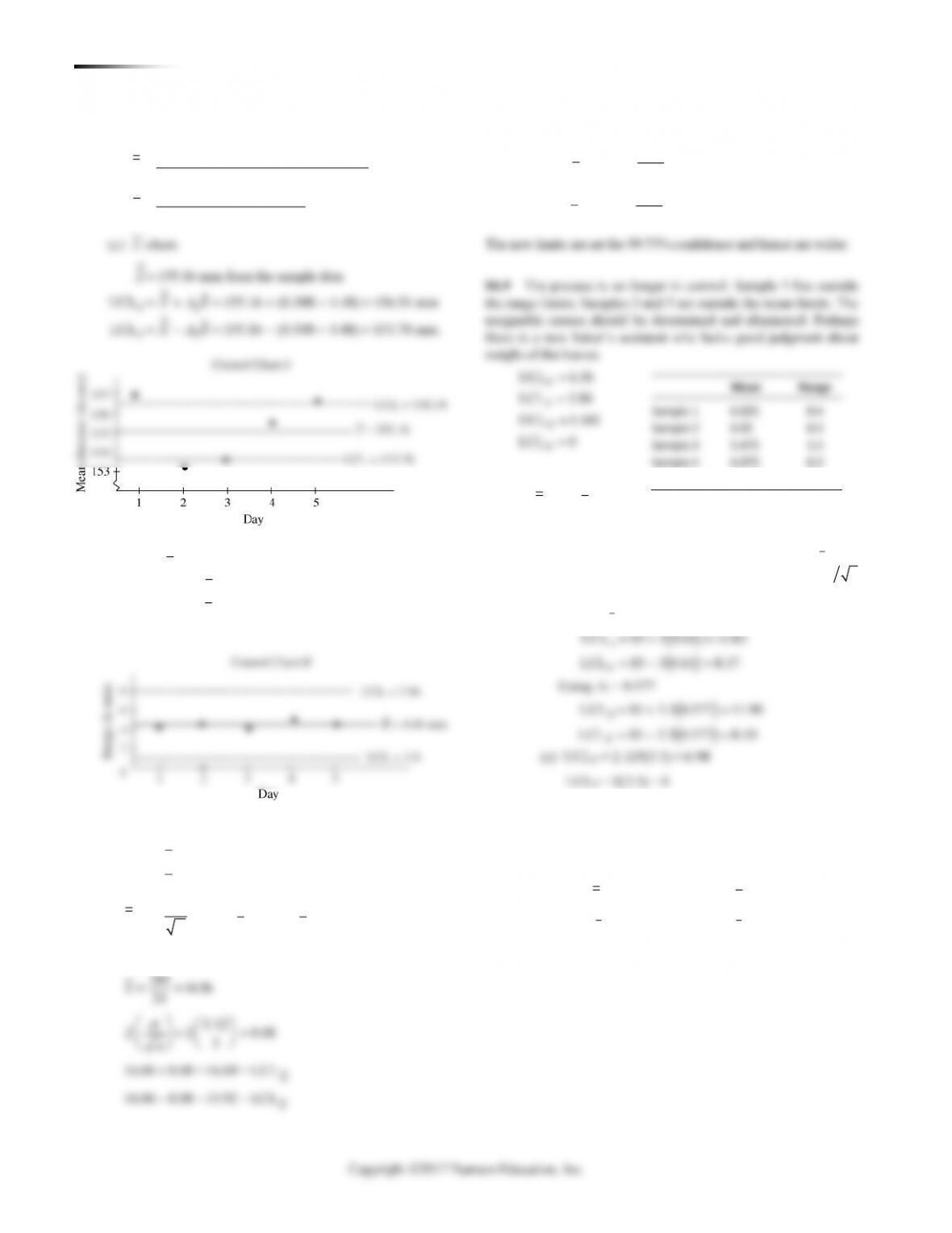
(b) Yes, the process appears to be under control. Samples
26–30 stayed within the boundaries of the upper and
lower control limits for both
X
and R charts.
(c) The observed lifetimes have a mean of approximately
50 hours, which supports the claim made by West Battery
Corp. However, the variance from the mean needs to be
controlled and reduced. Lifetimes should deviate from the
mean by no more than 5 hours (10% of the variance).
= + = + =
= − = − = −
UCL 6 3(2.45) 13.35
LCL 6 3(2.45) 1.35, or 0
c
c
c z c
c z c
36 6,
6=
3 4 = 4 + 3(2) = 10.
4. UCL 4c= = +
c-Chart for Test Errors
c-Chart for Number of Nonconformities
94 SUPPLEMENT 6 ST AT I ST I CA L PR OC ES S CO N TR O L
Sample
Late Flights
Percentage of
Late Flights
Percentage
(n/100)
in Sample
Late Flights (n/100)*
Sample
in Sample
of Late Flights
1
2
0.02
16
2
0.02
2
4
0.04
17
3
0.03
3
10
0.10
18
7
0.07
4
4
0.04
19
3
0.03
5
1
0.01
20
2
0.02
6
21
3
0.03
7
22
7
0.07
8
9
23
4
0.04
9
11
24
3
0.03
0
0.00
25
2
0.02
3
0.03
26
2
0.02
27
0
0.00
2
0.02
28
1
0.01
2
0.02
29
3
0.03
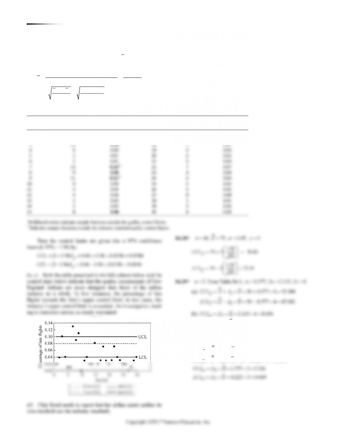
S6.27
(a) The overall percentage of late flights
()p
and the control
limits are developed as follows:
Total number of late flights 120 0.04
Number of samples Sample size 30 100
(1 ) 0.04 0.96
ˆ0.0196
100
= = =
−
= = =
p
p
pp
n
Table for Problem S6.27
SUPPLEMENT 6 ST AT ISTIC AL PROC ES S CO N T R O L 95
S6.31*
Sample
X
R
Sample
X
R
Sample
X
R
1
63.5
2.0
10
63.5
1.3
19
63.8
1.3
2
63.6
1.0
11
63.3
1.8
20
63.5
1.6
3
63.7
1.7
12
63.2
1.0
21
63.9
1.0
4
63.9
0.9
13
63.6
1.8
22
63.2
1.8
5
63.4
1.2
14
63.3
1.5
23
63.3
1.7
6
63.0
1.6
15
63.4
1.7
24
64.0
2.0
7
63.2
1.8
16
63.4
1.4
25
63.4
1.5
8
63.3
1.3
17
63.5
1.1
9
63.7
1.6
18
63.6
1.8
= = =
= = =
2 4 3
63.49, 1.5, 4. From Table S6.1,
0.729, 2.282, 0.0.
X R n
A D D
2
2
4
3
63.49 0.729 1.5 64.58
63.49 0.729 1.5 62.40
2.282 1.5 3.423
0 1.5 0
X
X
R
R
UCL X A R
LCL X A R
UCL D R
LCR D R
= + = + =
= − = − =
= = =
= = =
The process is in control.
S6.33*
Desired Desired
3.5, 50, 6R X n= = =
= + = + =
= − = − =
= = =
= = =
2
2
3
4
50 0.483 3.5 51.69
50 0.483 3.5 48.31
2.004 3.5 7.014
0 3.5 0
X
X
R
R
UCL X A R
LCL X A R
UCL D R
LCL D R
The smallest sample range is 1, and the largest 6. Both are
well within the control limits.
The smallest average is 47, and the largest 57. Both are
outside the proper control limits.
Therefore, although the range is within the limits, the average is
outside the limits, and apparently increasing. Immediate action is
needed to correct the problem and get the average within the control
limits again.
S6.34* 0.51
_ _ _ _ _ _ _ _ _ _ _ _ _ _ _ _ _ 0.505 drill bit (largest)
_ _ _ _ _ _ _ _ _ _ _ _ _ _ _ _ _ 0.495 drill bit (smallest)
0.49
0.505 – 0.49 = 0.015, 0.015/0.00017 = 88 holes within
standard
0.495 – 0.49 = 0.005, 0.005/0.00017 = 29 holes within
standard
Any one drill bit should produce at least 29 holes that meet
tolerance but no more than 88 holes before being replaced.
(1 )
3
(1 )
3
−
=+
−
=−
pp
UCL p
pn
pp
LCL p
pn
S6.35 *
Percent
n = 200
Defective (p)
1 – p
_
(1 )/p p n
p
LCL
p
U CL
0.01
0.99
0.0070
0.0
0.0310
0.02
0.98
0.0099
0.0
0.0497
0.03
0.97
0.0121
0.0
0.0663
0.04
0.96
0.0139
0.0
0.0817
0.05
0.95
0.0154
0.0038
0.0962
0.06
0.94
0.0168
0.0096
0.1104
0.07
0.93
0.0180
0.0160
0.1240
0.08
0.92
0.0192
0.0224
0.1376
0.09
0.91
0.0202
0.0294
0.1506
0.10
0.90
0.0212
0.0364
0.1636
96 SUPPLEMENT 6 ST AT I ST I CA L PR OC ES S CO N TR O L
(1 )
3
(1 )
3
0.011 0.989
0.011 3 0.0209
1000
0.011 0.989
0.011 3 0.0011
1000
−
=+
−
=−
= + =
= − =
p
p
p
p
pp
UCL p n
pp
LCL p n
UCL
LCL
S6.36 *
1
21
0.105
Y
2
8
0.04
Y
3
18
0.09
Y
4
14
0.07
Y
5
20
0.1
Y
6
12
0.06
Y
19
21
0.105
Y
20
26
0.13
Y
21
28
0.14
Y
22
22
0.11
Y
23
17
0.085
Y
24
14
0.07
Y
25
12
0.06
Y
Std. Deviation of p = 0.020477
7
29
0.145
Y
8
24
0.12
Y
9
16
0.08
Y
10
20
0.1
Y
11
12
0.06
Y
12
7
0.035
Y
13
13
0.065
Y
14
24
0.12
Y
15
24
0.12
Y
16
32
0.16
N
17
12
0.06
Y
18
16
0.08
Y
SUPPLEMENT 6 ST AT ISTIC AL PROC ES S CO N T R O L 97
=
= = =
p
Difference between upper and lower specifications
C6
.6 .6 1.0
6(.1) .6
S6.40
This process is barely capable.
−
=
−
= = =
p
Upper specification Lower specification
C6
2,400 1,600 800 1.33
6(100) 600
S6.41
pk
C min ,
33
2,400 1,800 1,800 1,600
min ,
3(100) 3(100)
min [2.00, 0.67] = 0.67
USL x x LSL
−−
=
−−
=
=
The Cp tells us the machine’s variability is acceptable
relative to the range of tolerance limits. But the Cpk tells us the
distribution of output is too close to the lower specification and
will produce chips whose lives are too short.
−−
=
==
=
pk
pk
8.135 8.00 8.00 7.865
C min of , or
(3)(0.04) (3)(0.04)
0.135 0.135
1.125, 1.125
0.12 0.12
Therefore, C 1.125.
S6.42
The process is centered and will produce within the specified
Upper tolerance limit
Lower tolerance limit
Standard deviation
S6.47*
Time
Box 1
Box 2
Box 3
Box 4
Average
9 AM
9.8
10.4
9.9
10.3
10.1
10 AM
10.1
10.2
9.9
9.8
10.0
11 AM
9.9
10.5
10.3
10.1
10.2
12 PM
9.7
9.8
10.3
10.2
10.0
1 PM
9.7
10.1
9.9
9.9
9.9
Average=
10.04
Std. Dev. =
0.11
10.1 10 10 9.9
0.3 and 0.3
(3)(0.11) (3)(0.11)
−−
==
As 0.3 is less than 1, the process will not produce within the
specified tolerance.
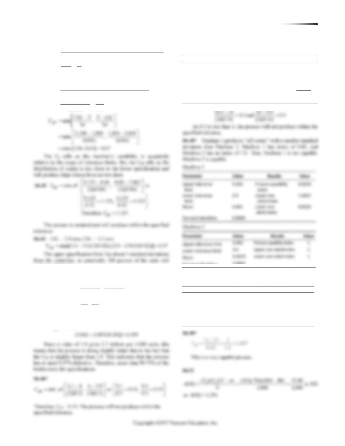
S6.48* Machine 1 produces “off–center” with a smaller standard
deviation than Machine 2. Machine 1 has index of 0.83, and
Machine 2 has an index of 1.0. Thus, Machine 1 is not capable.
Machine 2 is capable.
Machine 1
Parameter
Value
Results
Value
Upper tolerance
0.403
Process capability
0.8333
limit
index
Lower tolerance
0.4
Upper one
1.6667
limit
sided index
Mean
0.401
Lower one
0.8333
sided index
Standard deviation
0.0004
98 SUPPLEMENT 6 ST AT I ST I CA L PR OC ES S CO N TR O L
S6.52
( )( )( – ) (.04)(.57)(500 – 60) 10.0
AOQ = .02
500 500
AOQ 2.0%
da
P P N n
N= = =
=
Time
Ave
Low
High
Ave
Low
High
Ave
Low
High
4:00
50.3
49.2
52.7
47.2
45.3
50.9
50.0
49.1
50.6
5:00
51.4
50.0
55.3
46.8
44.1
49.0
45.2
51.2
6:00
51.6
49.2
54.7
46.8
41.0
51.2
44.0
49.7
7:00
51.8
50.0
55.6
50.0
46.2
51.7
44.4
50.0
8:00
51.0
48.6
53.2
47.4
44.0
48.7
46.6
48.9
Time
Ave
Low
High
Ave
Low
High
Ave
Low
High
10:00
49.2
46.1
50.7
46.6
50.2
49.2
48.1
50.7
11:00
49.0
46.3
50.8
48.6
47.0
50.0
47.0
50.8
12:00
45.4
50.2
49.8
48.2
50.4
46.4
49.2
44.3
49.7
49.6
48.4
51.7
46.8
49.0
44.1
49.6
50.0
49.0
52.2
48.8
47.2
51.4
45.2
49.0
50.0
49.2
50.0
49.6
49.0
50.6
49.1
46.3
50.5
51.0
50.5
51.5
5:00
47.1
49.6
44.1
49.7
50.5
50.0
51.9
1:00
49.0
46.4
50.0
50.1
49.4
53.6
48.9
47.6
51.2
Evening Shift
Time
Ave
Low
High
Ave
Low
High
Ave
Low
High
2:00
49.0
46.0
50.6
49.7
48.6
51.0
49.8
48.4
51.0
3:00
49.8
48.2
50.8
48.4
47.2
51.7
49.8
48.8
50.8
SUPPLEMENT 6 ST AT ISTIC AL PROC ES S CO N T R O L 99
1
2
The immediate problem, however, must be corrected by additional
training, bag weight monitoring, and weight-feeder adjustments.
Short-run declines in bag output may be necessary to achieve
acceptable bag weights.
AACSB: Application of knowledge
VIDEO CASE STUDIES
These videos have been created specifically for this text to
supplement the cases below.
FRITO-LAY’S QUALITY-CONTROLLED
POTATO CHIPS
Note to instructors: Here is a real-world case of a company whose
products are known to every student. We suggest you show this
AACSB: Application of knowledge
3. Quality drives this consumer product. The taste of each chip
or other snack must be the same every bite. The bags must be
identical in weight and appearance. The product must be fresh.
Every step in production—from farm to factory—needs to meet
AACSB: Application of knowledge
2. Many options in any restaurant exist for fishbone analysis.
These include customer satisfaction, employee performance, meal
quality, and delivery quality. In the solutions of Chapter 6, we
presented several fishbone charts that can provide a starting point
for quality analysis in a restaurant:
◼ For the dissatisfied restaurant customer, see Solution 6.8,
“A Dissatisfied Airline Customer”
100 SUPPLEMENT 6 STAT IS TIC AL PROC ES S CO N T R O L
Sample 11 warrants some evaluation, but the report should sug-
gest an excellent process, and you tell the vendor to keep up the
good work.
LO S6.3: Build x-bar charts and R-charts
AACSB: Application of knowledge
ADDITIONAL CASE STUDY
(AVAILABLE IN MYOMLAB)
GREEN RIVER CHEMICAL CO.
This is a very straightforward case. Running software to analyze
the data will generate the
-chart asX