48 CHAPTER 4 FO R E C A S T I N G
4.46 (a)
x
y
xy
x2
16
330
5,280
256
12
270
3,240
144
14
300
4,200
196
2 2 2
20
920 4(15)
b
x nx
= = = =
− −
additional $18 in bar sales.
4.47 Y = 7.5 + 3.5X1 + 4.5X2 + 2.5X3
1
58.3
36
3,398.9
1,296
2,098.8
2
61.1
33
3,733.2
1,089
2,016.3
4.48 (a)
ˆ
Y
= 13,473 + 37.65(1860) = 83,502
(b) The predicted selling price is $83,502, but this is the
average price for a house of this size. There are other
factors besides square footage that will impact the sell-
ing price of a house. If such a house sold for $95,000,
then these other factors could be contributing to the
additional value.
(c) Some other quantitative variables would be age of the
4.49 (a) Given: Y = 90 + 48.5X1 + 0.4X2 where:
1
2
expected travel cost
number of days on the road
distance traveled, in miles
0.68 (coefficient of correlation)
Y
X
X
r
=
=
=
=
(c) A number of other variables should be included, such as:
1. The type of travel (air or car)
4.50 (a) Least-squares equation: Y = –0.158 + 0.1308X
4.51
Crime
Patients
Year
Rate X
Y
X2
Y2
XY
3
73.4
40
5,387.6
1,600
2,936.0
4
75.7
41
5,730.5
1,681
3,103.7
5
81.1
40
6,577.2
1,600
3,244.0
6
89.0
55
7,921.0
3,025
4,895.0
7
101.1
60
10,221.2
3,600
6,066.0
8
94.8
54
8,987.0
2,916
5,119.2
9
103.3
58
10,670.9
3,364
5,991.4
10
116.2
61
13,502.4
3,721
7,088.2
Column totals
854.0
478
76,129.9
23,892
42,558.6
2
42558.6 10 85.4 47.8 42558.6 40821.2
76129.9 72931.6
76129.9 10 85.4
1737.4 0.543
3197.3
47.8 0.543 85.4 1.43
b
a
− −
==
−
−
==
= − =
50 CHAPTER 4 FO R E C A ST I N G
As an indication of the usefulness of this relationship, we can
calculate the correlation coefficient:
()()
22
22
22
13 20299.5 6885 36.96
13 3857893 6885 13 110.26 36.96
263893.5 254469.6
50152609 47403225 1433.4 1366.0
9423.9
2749384 67.0
9423.9 0.69
1658.13 8.21
n XY X Y
r
n X X n Y Y
−
=
− −
−
=
− −
−
=−−
=
==
2
2
0.479r=
A correlation coefficient of 0.692 is not particularly high. The
coefficient of determination, r2, indicates that the model explains
only 47.9% of the overall variation. Therefore, although the model
does provide an estimate of GPA, there is considerable variation
in GPA, which is as yet unexplained. For
(b) 350: 1.03 0.0034 350 2.22
(c) 800: 1.03 0.0034 800 3.75
XY
XY
= = + =
= = + =
Note: When solving this problem, care must be taken to interpret
significant digits. Also note that X = 800 is outside the range of
the data set used to determine the regression relationship, so
caution is advised.
4.54 (a)
Quarter
Contracts X
Sales Y
X2
Y2
XY
1
153
8
23,409
64
1,224
2
172
10
29,584
100
1,720
3
197
15
38,809
225
2,955
4
178
9
31,684
81
1,602
5
185
12
34,225
144
2,220
6
199
13
39,601
169
2,587
7
205
12
42,025
144
2,460
8
226
16
51,076
256
3,616
Totals
1,515
95
290,413
1,183
18,384
Average
189.375
11.875
b = (18,384 – 8 × 189.375 × 11.875)/(290,413 – 8 × 189.375
× 189.375) = 0.1121
a = 11.875 – 0.1121 × 189.375 = –9.3495
Sales ( y) = –9.349 + 0.1121 (Contracts)
(b)
22
(8 18,384 1,515 95)
((8 290,413 1,515 )(8 1,183 95 ))
0.8963
= −
− −
=
r
4.55* (a) 35 + 20(80) + 50(3.0) = 1,785
(b) 35 + 20(70) + 50(2.5) = 1,560
4.56* Given: X = 15, Y = 20, XY = 70, X2 = 55, Y2 = 130,
X
= 3,
Y
= 4
22
2
(a)
70 5 3 4 70 60 10 1
55 45 10
55 5 3
4 1 3 4 3 1
11
−
=−
=−
− −
= = = =
−
−
= − = − =
=+
XY nXY
b
X nX
a Y bX
b
a
YX
(b) Correlation coefficient:
()()
22
22
22
5 70 15 20
5 55 15 5 130 20
350 300 50
50 250
275 225 650 400
50 0.45
111.80
n XY X Y
r
n X X n Y Y
−
=
− −
−
=
− −
−
==
−−
==
The correlation coefficient indicates that there is a positive
correlation between bank deposits and consumer price indices in
Birmingham, Alabama—i.e., as one variable tends to increase
(or decrease), the other tends to increase (or decrease).
(c) Standard error of the estimate:
2130 1 20 1 70
23
130 20 70 40 13.3 3.65
33
yx
Y a Y b XY
Sn
− − − −
==
−
−−
= = = =
4.57*
X
Y
X2
Y2
XY
2
4
4
16
8
1
1
1
1
1
4
4
16
16
16
5
6
25
36
30
3
5
9
25
15
Column totals
15
20
55
94
70
Given: Y = a + bX where:
22
XY nXY
b
X nX
a Y bX
−
=−
=−
and X = 15, Y = 20, XY = 70, X2 = 55, Y2 = 94,
X
= 3,
Y
CHAPTER 4 FO R E C A ST I N G 51
and Y = 1.0 + 1.0X. The correlation coefficient:
()()
22
22
22
5 70 15 20 350 300
275 225 470 400
5 55 15 5 94 20
50 50 0.845
59.16
50 70
n XY X Y
r
n X X n Y Y
−
=
− −
− −
==
−−
− −
= = =
9
22
+3.51
10.94
19.88
2.21
5
20
19.19
+0.81
11.75
20.69
2.07
5.7
15
19.35
–4.35
7.40
25.04
2.28
3.2
22
18.48
+3.52
10.92
28.56
2.38
4.6
94 20 70 1.333 1.15
3
−−
= = =
4.58* Using software, the regression equation is: Games lost =
4.59 (a, b)
Period
Demand
Forecast
Error
Running Sum
|Error|
1
20
20
0.00
0.00
0.00
2
21
20
1.00
1.00
1.00
3
28
20.5
7.50
8.50
7.50
4
37
24.25
21.25
12.75
5
25
30.63
–5.63
15.63
5.63
6
29
27.81
1.19
16.82
1.19
7
36
28.41
7.59
24.41
7.59
8
22
32.20
–10.20
14.21
10.20
9
25
27.11
–2.10
12.10
2.10
10
28
26.05
1.95
14.05
1.95
MAD
5.00
(c) Cumulative error = 14.05; MAD = 5 Tracking = 14.05/5 = 2.82
4.60
1
()
Tracking signal M AD
n
tt
t
AF
=
−
=
Month
At
Ft
|At – Ft |
(At – Ft)
May
100
100
0
0
June
104
24
July
110
11
11
August
115
101
14
14
September
105
104
1
1
October
110
104
6
6
November
125
105
20
20
December
120
109
11
11
Sum: 87
Sum: 39
10.875
4.61* (a)
Actual
Cumulative
Cum.
Tracking
Week
Miles
Forecast
Error
Error
|Error|
MAD
Signal
1
17
17.00
0.00
–
0.00
0
2
21
17.00
+4.00
4.00
4.00
2
2
3
19
17.80
+1.20
5.20
5.20
1.73
3
4
23
18.04
+4.96
10.16
10.16
2.54
4
5
18
19.03
–1.03
9.13
11.19
2.24
4
6
16
18.83
–2.83
6.30
14.02
2.34
2.7
7
20
18.26
+1.74
8.04
15.76
2.25
3.6
8
18
18.61
–0.61
7.43
16.37
2.05
3.6
(c) The cumulative error and tracking signals appear to
be consistently positive, and at week 10, the tracking
signal exceeds 5 MADs.
SOUTHWESTERN UNIVERSITY: B
This is the second in a series of integrated case studies that run
throughout the text.
1. One way to address the case is with separate forecasting models
Forecasts
Game
Model
2016
2017
R2
1
y = 30,713 + 2,534x
48,453
50,988
0.92
2
y = 37,640 + 2,146x
52,660
54,806
0.90
3
y = 36,940 + 1,560x
47,860
49,420
0.91
4
y = 22,567 + 2,143x
37,567
39,710
0.88
5
y = 30,440 + 3,146x
52,460
55,606
0.93
Total
239,000
250,530
(where y = attendance and x = time)
LO 4.3: Apply the naïve, moving-average, exponential smooth-
ing, and trend methods
AACSB: Analytical thinking
2. Revenue in 2016 = (239,000) ($50/ticket) = $11,950,000
3. In games 2 and 5, the forecast for 2017 exceeds stadium ca-
52 CHAPTER 4 FO R E C A ST I N G
1
2
VIDEO CASE STUDIES
FORECASTING TICKET REVENUE FOR
1. Regression model using “day of the week” as independent
2. Regression model using “rating of the opponent” as inde-
3. Using the multiple regression model in the case:
Revenue = $14,996 + 10,801 (4) + 23,379 (3) + 10,784 (3)
= $160,743
2
17
24
408
3
25
27
675
4
25
32
1,024
800
5
35
29
1,225
1,015
6
35
37
1,225
1,369
1,295
7
45
43
2,025
1,849
1,935
AACSB: Analytical thinking
4. Time of day for game, other competing sports events within
FORECASTING AT HARD ROCK CAFE
There is a short video (8 minutes) available from Pearson and
filmed specifically for this text that supplements this case.
1. Hard Rock case uses forecasting for (1) sales (guest counts)
at cafes, (2) retail sales, (3) banquet sales, (4) concert sales, (5) eval-
2. The POS system captures all the basic sales data needed to
drive individual cafe’s scheduling/ordering. It also is aggregated
at corporate HQ. Each entrée sold is counted as one guest at a
This system actually protects managers from large sales variations
outside their control. One could also justify a 50%–30%–20%
4. Other predictors of cafe sales could include season of year
5. Y = a + bx
Month
Advertising X
Guest Count Y
X2
Y2
XY
1
14
21
196
441
294
9
60
54
3,600
2,916
3,240
10
60
66
3,600
4,356
3,960
Totals
366
376
15,910
15,950
15,772
Average
36.6
37.6
At $65,000; y = 8.3 + .8 (65) = 8.3 + 52 = 60.3, or 60,300 guests.
For the instructor who asks other questions than this one:
r2 = 0.8869
Std. error = 5.062
LO 4.6: Conduct a regression and correlation analysis
CHAPTER 4 FO R E C A ST I N G 53
ADDITIONAL CASE STUDIES
(available in MyOMLab)
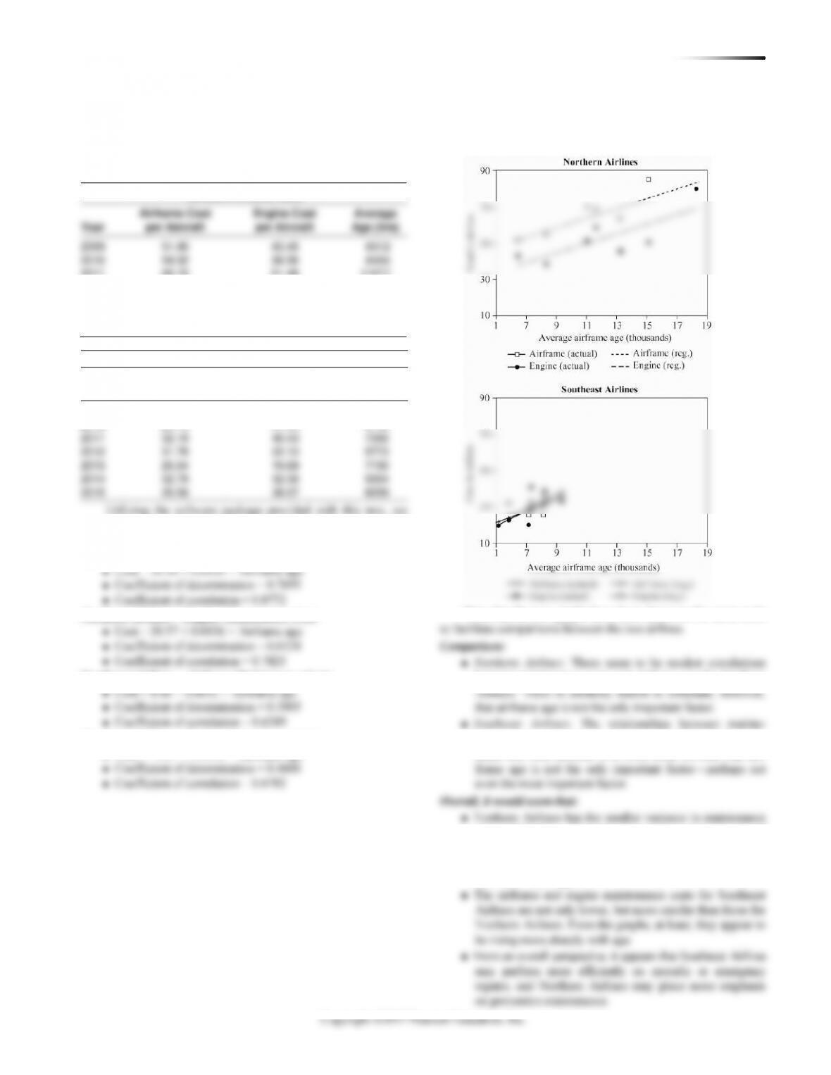
THE NORTH-SOUTH AIRLINES
Northern Airlines Data
Airframe Cost
Engine Cost
Average
Year
per Aircraft
per Aircraft
Age (hrs)
2009
51.80
43.49
6512
2010
54.92
38.58
8404
2011
69.70
51.48
11077
2012
68.90
58.72
11717
2013
63.72
45.47
13275
2014
84.73
50.26
15215
2015
78.74
79.60
18390
Southeast Airlines Data
Airframe Cost
Engine Cost
Average
Year
per Aircraft
per Aircraft
Age (hrs)
2009
13.29
18.86
5107
2010
25.15
31.55
8145
2011
32.18
40.43
7360
2012
31.78
22.10
5773
2013
25.34
19.69
7150
2014
32.78
32.58
9364
2015
35.56
38.07
8259
Utilizing the software package provided with this text, we
can develop the following regression equations for the variables
of interest:
Northern Airlines—Airframe Maintenance Cost:
Southeast Airlines—Airframe Maintenance Cost:
Southeast Airlines—Engine Maintenance Cost;
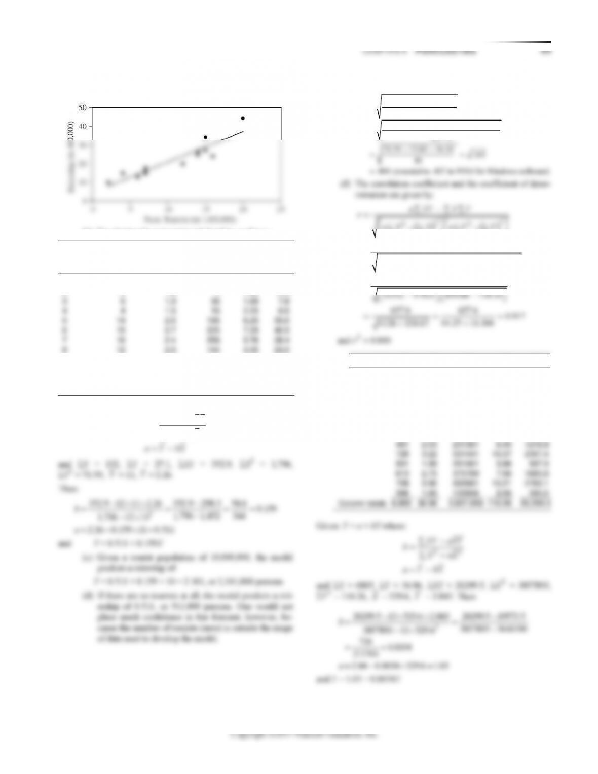
The following graphs portray both the actual data and the
regression lines for airframe and engine maintenance costs for
both airlines.
between maintenance costs and airframe age for Northern
nance costs and airframe age for Southeast Airlines are
costs—indicating that its day-to-day management of
maintenance is working pretty well.
◼ Maintenance costs seem to be more a function of airline
than of airframe age.
54 CHAPTER 4 FO R E C A ST I N G
Ms. Young’s report should conclude that:
◼ There is evidence to suggest that maintenance costs could
be made to be a function of airframe age by implementing
more effective management practices.
◼ The difference between maintenance procedures of the two
DIGITAL CELL PHONE, INC.
1. A plot of the data indicates a linear trend (least squares) mod-
el might be appropriate for forecasting. Using linear trend you
obtain the following:
x
y
x2
xy
y2
1
480
1
480
230,400
2
436
4
872
190,096
3
482
9
1,446
232,324
5
458
25
2,290
209,464
6
489
36
2,934
239,121
7
498
49
3,486
248,004
8
430
64
3,440
184,900
9
444
81
3,996
197,136
10
496
100
4,960
246,016
11
487
121
5,357
237,169
12
525
144
6,300
275,625
13
575
169
7,475
330,625
14
527
196
7,378
277,729
15
540
225
8,100
291,600
16
502
256
8,032
252,004
17
508
289
8,636
258,064
18
573
324
10,314
328,329
19
508
361
9,652
258,064
20
498
400
9,960
248,004
21
485
441
10,185
235,225
30
605
900
18,150
366,025
22
526
484
11,572
276,676
23
552
529
12,696
304,704
24
587
576
14,088
344,569
25
608
625
15,200
369,664
26
597
676
15,522
356,409
27
612
729
16,524
374,544
28
603
784
16,884
363,609
29
628
841
18,212
394,384
31
627
961
19,437
393,129
32
578
1,024
18,496
334,084
33
585
1,089
19,305
342,225
34
581
1,156
19,754
337,561
35
632
1,225
22,120
399,424
36
656
1,296
23,616
430,336
Totals
666
19,366
16,206
378,661
10,558,246
=
[139,860
=
][5,054,900] 706,978,314,000
The student should report the linear trend results, but deflate
the forecast obtained based on qualitative information about
industry and technology trends.
Because there is limited seasonality in the data, the linear
2. Four approaches to decomposition of the Digital Cell Phone
data can address seasonality, as follows:
(a) Multiplicative seasonal model,
Cases = 443.87 + 5.08 (time), r2 = .85, MAD = 20.89
(b) Multiplicative Seasonal Model, with centered moving averages
(CMA), which is not covered in our text but can be seen in