CHAPTER 4 FO R E C A ST I N G 41
2 2 2
650 4(2.5)(55) 650 550
30 25
30 4(2.5)
100 20
5
55 (20)(2.5)
5
xy nx y
b
x nx
a y bx
− − −
= = = −
− −
==
=−
=−
=
The regression line is y = 5 + 20x. The forecast for May (x = 5) is
y = 5 + 20(5) = 105.
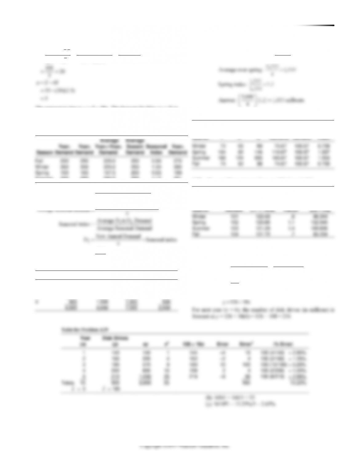
4.25
Season
Year1
Demand
Year2
Demand
Average
Year1–Year2
Demand
Average
Season
Demand
Seasonal
Index
Year3
Demand
Fall
200
250
225.0
250
0.90
270
Winter
350
300
325.0
250
1.30
390
Spring
150
165
157.5
250
0.63
189
Summer
300
285
292.5
250
1.17
351
12 12
12
12
3
Average to Demand Demand
2
Demand for season
Sum of Ave to Demand
Average seasonal demand 4
Average to Demand
Seasonal index = Average Seasonal Demand
New Annual Demand S
4
Yr Yr Yr Yr
Yr Yr
Yr Yr
Yr
+
=
=
=
easonal index
1200 Seasonal index
4
=
4.26
Year
Winter
Spring
Summer
Fall
1
1,400
1,500
1,000
600
2
1,200
1,400
2,100
750
3
1,000
1,600
2,000
650
4
900
1,500
1,900
500
4,500
6,000
7,000
2,500
Average over all seasons:
Average over spring:
Spring index:
5,600
Answer: sailboats
4
20,000 1,250
16
6,000 1,500
4
1,500 1.2
1,250
(1.2) 1,680
=
=
=
=
4.27
Quarter
Year
1
Year
2
Year
3
Average
Demand
Average
Quarterly
Demand
Seasonal
Index
Winter
73
65
89
75.67
106.67
0.709
Spring
104
82
146
110.67
106.67
1.037
Summer
168
124
205
165.67
106.67
1.553
Fall
74
52
98
74.67
106.67
0.700
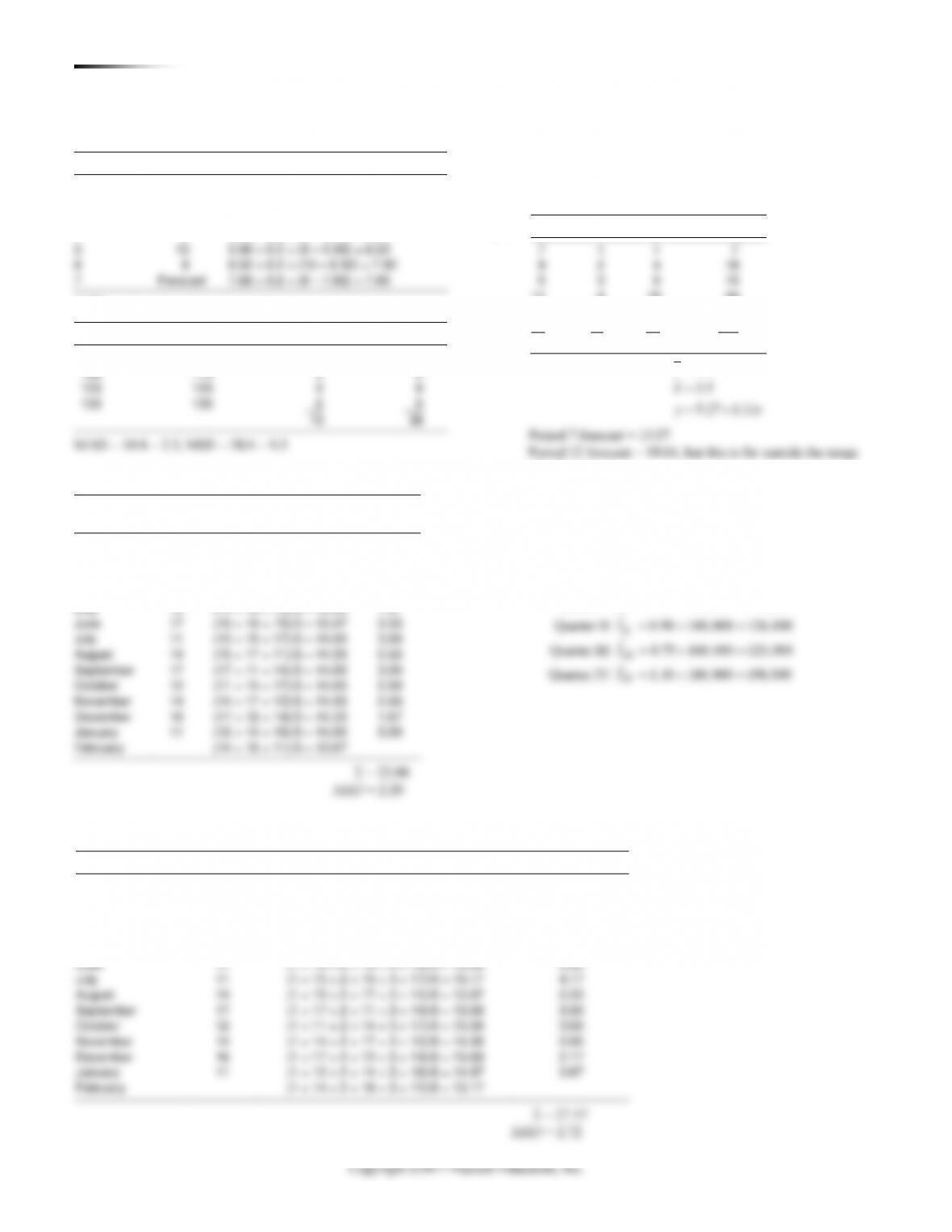
4.28 The year 26 quarter numbers are 101 through 104.
(5)
(2)
(3)
(4)
Adjusted
(1)
Quarter
Forecast
Seasonal
Forecast
Quarter
Number
(77 + .43Q)
Factor
[(3) × (4)]
Winter
101
120.43
.8
96.344
Spring
102
120.86
1.1
132.946
Summer
103
121.29
1.4
169.806
Fall
104
121.72
.7
85.204
4.29 (a) See the table below.
2
2,880 5(3)(180) 2,880 2,700
55 45
55 5(3)
180 18
10
180 3(18) 180 54 126
126 18
−−
==
−
−
==
= − = − =
=+
b
a
yx
Year
1
140
1
2
320
4
3
570
9
5
1,050
Totals
= 180
42 CHAPTER 4 FO R E C A ST I N G
4.30
Year X
Patients Y
X2
Y2
XY
1
36
1
1,296
36
2
33
4
1,089
66
3
40
9
1,600
120
4
41
16
1,681
164
5
40
25
1,600
200
6
55
36
3,025
330
7
60
49
3,600
420
8
54
64
2,916
432
9
58
81
3,364
522
10
61
100
3,721
610
55
478
385
23,892
2,900
Given: Y = a + bX where:
22
XY nXY
b
X nX
a Y bX
−
=−
=−
and X = 55, Y = 478, XY = 2900, X2 = 385, Y2 = 23892,
5.5, 47.8,XY==
Then:
− −
= = = =
−
−
= − =
2
2,900 10 5.5 47.8 2,900 2,629 271 3.28
385 302.5 82.5
385 10 5.5
47.8 3.28 5.5 29.76
b
a
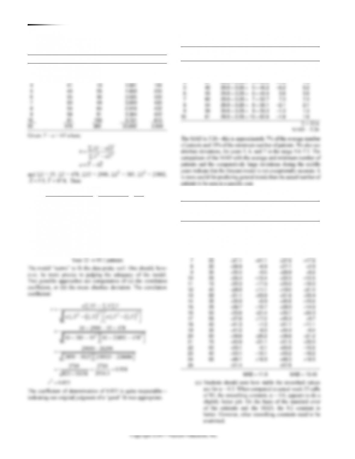
and Y = 29.76 + 3.28X. For:
11: 29.76 3.28 11 65.8
12: 29.76 3.28 12 69.1
XY
XY
= = + =
= = + =
Therefore:
Year 11 → 65.8 patients
7
20
+41.1
–21.1
+37.6
–17.6
8
30
+36.9
–6.9
+27.1
+2.9
9
35
+35.5
–0.5
+28.8
+6.2
20
+35.4
–15.4
+32.5
–12.5
15
+32.3
–17.3
+25.0
–10.0
40
+28.9
+11.1
+19.0
+21.0
55
+31.1
+23.9
+31.6
+23.4
35
+35.9
–0.9
+45.6
–10.6
25
+36.7
–10.7
+39.3
–14.3
55
+33.6
+21.4
+30.7
+24.3
55
+37.8
+17.2
+45.3
+9.7
40
+41.3
–1.3
+51.1
–11.1
35
+41.0
–6.0
+44.4
–9.4
60
+39.8
+38.8
+21.2
75
+43.9
+31.1
+51.5
+23.5
50
+50.1
–0.1
+65.6
–15.6
40
+50.1
–10.1
+56.2
–16.2
65
+48.1
+16.9
+46.5
+18.5
Year
Patients
Trend
Absolute
X
Y
Forecast
Deviation
Deviation
1
36
29.8 + 3.28 × 1 = 33.1
2.9
2.9
2
33
29.8 + 3.28 × 2 = 36.3
–3.3
3.3
3
40
29.8 + 3.28 × 3 = 39.6
0.4
0.4
4
41
29.8 + 3.28 × 4 = 42.9
–1.9
1.9
5
40
29.8 + 3.28 × 5 = 46.2
–6.2
6.2
6
55
29.8 + 3.28 × 6 = 49.4
5.6
5.6
7
60
29.8 + 3.28 × 7 = 52.7
7.3
7.3
8
54
29.8 + 3.28 × 8 = 56.1
–2.1
2.1
9
58
29.8 + 3.28 × 9 = 59.3
–1.3
1.3
10
61
29.8 + 3.28 × 10 = 62.6
–1.6
1.6
= 32.6
MAD = 3.26
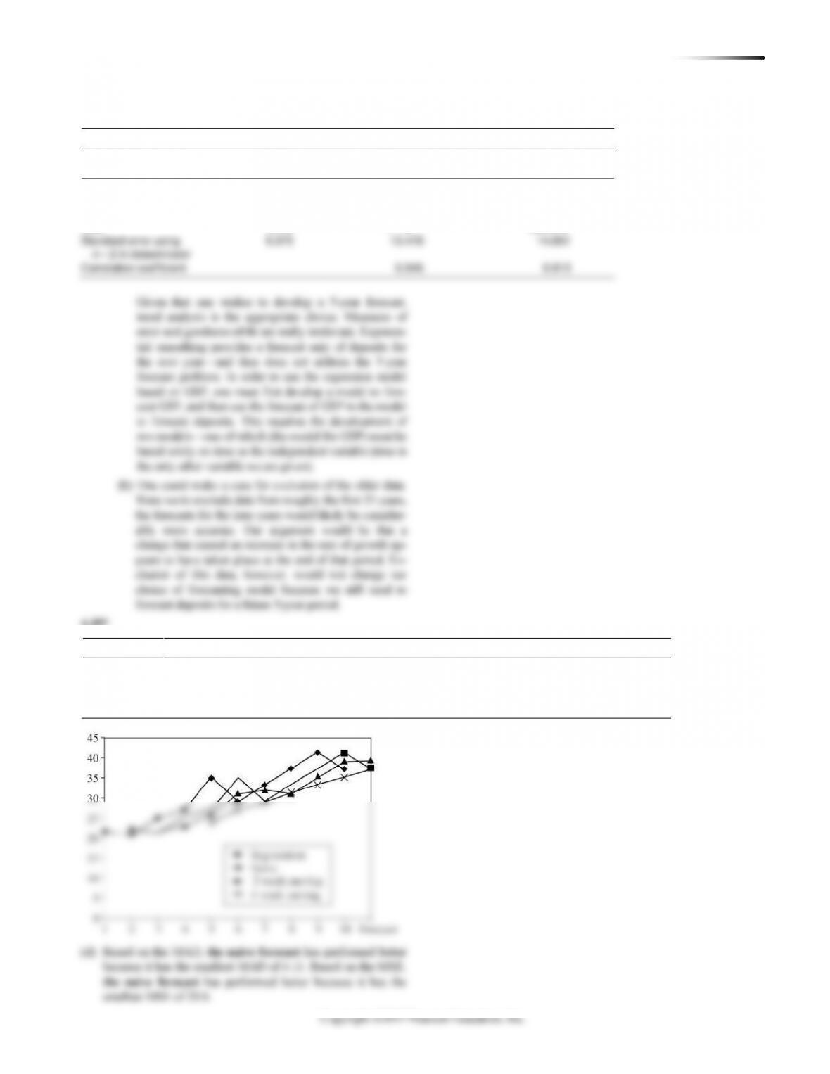
The MAD is 3.26—this is approximately 7% of the average number
of patients and 10% of the minimum number of patients. We also see
absolute deviations, for years 5, 6, and 7 in the range 5.6–7.3. The
comparison of the MAD with the average and minimum number of
patients and the comparatively large deviations during the middle
years indicate that the forecast model is not exceptionally accurate. It
is more useful for predicting general trends than the actual number of
patients to be seen in a specific year.
4.31 (a) and (b) See the following table:
Actual
Smoothed
Smoothed
Week
Value
Value
Forecast
Value
Forecast
t
A(t)
Ft ( = 0.2)
Error
Ft ( = 0.6)
Error
1
50
+50.0
+0.0
+50.0
+0.0
2
35
+50.0
–15.0
+50.0
–15.0
3
25
+47.0
–22.0
+41.0
–16.0
4
40
+42.6
–2.6
+31.4
+8.6
5
45
+42.1
–2.9
+36.6
+8.4
6
35
+42.7
–7.7
+41.6
–6.6
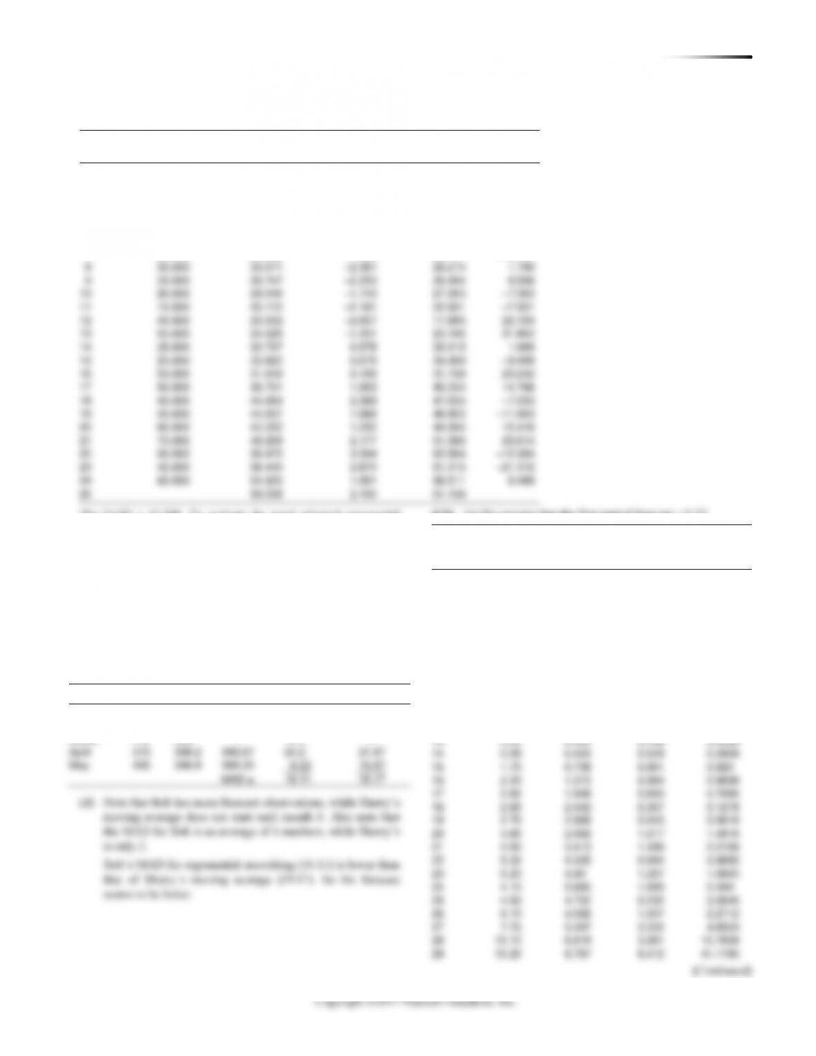
CHAPTER 4 FO R E C A ST I N G 43
The MAD = 12.208. To evaluate the trend adjusted exponential
smoothing model, actual week 25 calls are compared to the forecast
value. The model appears to be producing a MAD approximately
mid–range between that given by simple exponential smoothing
using = 0.2 and = 0.6. Trend adjustment does not appear to give
any significant improvement.
4.33 (a) There is not a strong linear trend in sales over time.
(b, c) Bob wants to forecast by exponential smoothing (setting
February’s forecast equal to January’s sales) with alpha =
0.1. Sherry wants to use a 3-period moving average.
Sales
Bob
Sherry
Bob’s Error
Sherry’s Error
January
400
—
—
—
—
February
380
400
—
20.0
—
March
410
398
—
12.0
—
April
375
399.2
396.67
24.2
21.67
May
405
396.8
388.33
8.22
16.67
MAD =
16.11
19.17
(d) Note that Bob has more forecast observations, while Sherry’s
moving average does not start until month 4. Also note that
the MAD for Bob is an average of 4 numbers, while Sherry’s
is only 2.
Bob’s MAD for exponential smoothing (16.11) is lower than
that of Sherry’s moving average (19.17). So his forecast
seems to be better.
8
30.000
30.571
–2.361
28.210
1.790
9
35.000
28.747
–2.253
26.494
8.506
10
20.000
29.046
–1.743
27.303
–7.303
11
15.000
25.112
–2.181
22.931
–7.931
12
40.000
20.552
–2.657
17.895
22.105
13
55.000
24.526
–1.331
23.196
31.804
14
35.000
32.737
0.578
33.315
1.685
15
25.000
33.820
0.679
34.499
–9.499
16
55.000
31.649
0.109
31.758
23.242
17
55.000
38.731
1.503
40.234
14.766
18
40.000
44.664
2.389
47.053
–7.053
19
35.000
44.937
1.966
46.903
–11.903
20
60.000
43.332
1.252
44.584
15.416
21
75.000
49.209
2.177
51.386
23.614
22
50.000
58.470
3.594
62.064
–12.064
23
40.000
58.445
2.870
61.315
–21.315
24
65.000
54.920
1.591
56.511
8.489
4.34 (a) We assume that the first-period forecast = 0.25.
Method → Exponential Smoothing
0.6 =
Year
Deposits (Y)
Forecast
|Error|
Error2
1
0.25
0.25
0.00
0.00
2
0.24
0.25
0.01
0.0001
3
0.24
0.244
0.004
0.0000
4
0.26
0.241
0.018
0.0003
5
0.25
0.252
0.002
0.00
6
0.30
0.251
0.048
0.0023
7
0.31
0.280
0.029
0.0008
8
0.32
0.298
0.021
0.0004
9
0.24
0.311
0.071
0.0051
10
0.26
0.268
0.008
0.0000
11
0.25
0.263
0.013
0.0002
12
0.33
0.255
0.074
0.0055
13
0.50
0.300
0.199
0.0399
14
0.95
0.420
0.529
0.2808
15
1.70
0.738
0.961
0.925
16
2.30
1.315
0.984
0.9698
17
2.80
1.906
0.893
0.7990
18
2.80
2.442
0.357
0.1278
19
2.70
2.656
0.043
0.0018
20
3.90
2.682
1.217
1.4816
21
4.90
3.413
1.486
2.2108
22
5.30
4.305
0.994
0.9895
23
6.20
4.90
1.297
1.6845
24
4.10
5.680
1.580
2.499
25
4.50
4.732
0.232
0.0540
26
6.10
4.592
1.507
2.2712
27
7.70
5.497
2.202
4.8524
28
10.10
6.818
3.281
10.7658
29
15.20
8.787
6.412
41.1195
(Continued)
4.32
Week
Actual Value
Smoothed Value
Trend Estimate
Forecast
Forecast
t
At
Ft (
= 0.3)
Tt (
= 0.2)
FITt
Error
1
50.000
50.000
0.000
50.000
0.000
2
35.000
50.000
0.000
50.000
–15.000
3
25.000
45.500
–0.900
44.600
–19.600
4
40.000
38.720
–2.076
36.644
3.356
5
45.000
37.651
–1.875
35.776
9.224
6
35.000
38.543
–1.321
37.222
–2.222
7
20.000
36.555
–1.455
35.101
–15.101
44 CHAPTER 4 FO R E C A ST I N G
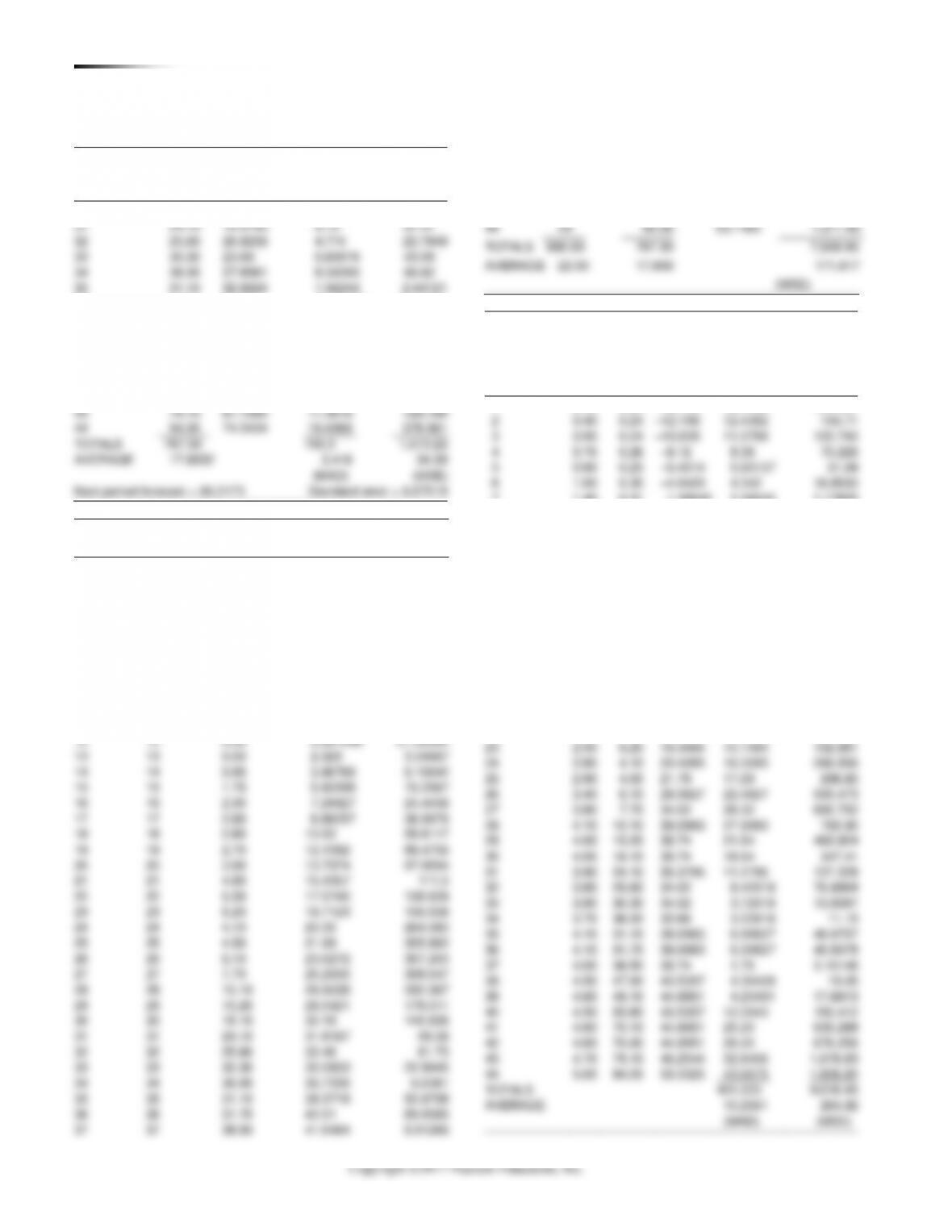
4.34 (a) (Continued)
Method → Exponential Smoothing
0.6 =
Year
Deposits (Y)
Forecast
|Error|
Error2
30
18.10
12.6350
5.46498
29.8660
31
24.10
15.9140
8.19
67.01
32
25.60
20.8256
4.774
22.7949
33
30.30
23.69
6.60976
43.69
34
36.00
27.6561
8.34390
69.62
35
31.10
32.6624
1.56244
2.44121
36
31.70
31.72
0.024975
0.000624
37
38.50
31.71
6.79
46.1042
38
47.90
35.784
12.116
146.798
39
49.10
43.0536
6.046
36.56
40
55.80
46.6814
9.11856
83.1481
41
70.10
52.1526
17.9474
322.11
42
70.90
62.9210
7.97897
63.66
43
79.10
67.7084
11.3916
129.768
44
94.00
74.5434
19.4566
378.561
TOTALS
787.30
150.3
1,513.22
AVERAGE
17.8932
3.416
34.39
(MAD)
(MSE)
Next period forecast = 86.2173
Standard error = 6.07519
Method → Linear Regression (Trend Analysis)
Year
Period (X)
Deposits (Y)
Forecast
Error2
1
1
0.25
–17.330
309.061
2
2
0.24
–15.692
253.823
3
3
0.24
–14.054
204.31
4
4
0.26
–12.415
160.662
5
5
0.25
–10.777
121.594
6
6
0.30
–9.1387
89.0883
7
7
0.31
–7.50
61.0019
8
8
0.32
–5.8621
38.2181
9
9
0.24
–4.2238
19.9254
10
10
0.26
–2.5855
8.09681
11
11
0.25
–0.947
1.43328
12
12
0.33
0.691098
0.130392
13
13
0.50
2.329
3.34667
14
14
0.95
3.96769
9.10642
15
15
1.70
5.60598
15.2567
16
16
2.30
7.24427
24.4458
17
17
2.80
8.88257
36.9976
18
18
2.80
10.52
59.6117
19
19
2.70
12.1592
89.4756
20
20
3.90
13.7974
97.9594
21
21
4.90
15.4357
111.0
22
22
5.30
17.0740
138.628
23
23
6.20
18.7123
156.558
24
24
4.10
20.35
264.083
25
25
4.50
21.99
305.862
26
26
6.10
23.6272
307.203
27
27
7.70
25.2655
308.547
28
28
10.10
26.9038
282.367
29
29
15.20
28.5421
178.011
30
30
18.10
30.18
145.936
31
31
24.10
31.8187
59.58
32
32
25.60
33.46
61.73
33
33
30.30
35.0953
22.9945
34
34
36.00
36.7336
0.5381
35
35
31.10
38.3718
52.8798
36
36
31.70
40.01
69.0585
37
37
38.50
41.6484
9.91266
38
38
47.90
43.2867
21.2823
39
39
49.10
44.9250
17.43
40
40
55.80
46.5633
85.3163
41
41
70.10
48.2016
479.54
42
42
70.90
49.84
443.528
43
43
79.10
51.4782
762.964
44
44
94.00
53.1165
1,671.46
TOTALS
990.00
787.30
7,559.95
AVERAGE
22.50
17.893
171.817
(MSE)
Method → Least squares–Simple Regression on GSP
(a)
(b)
–17.636
13.5936
Coefficients:
GSP
Deposits
Year
(X)
(Y)
Forecast
|Error|
Error2
1
0.40
0.25
–12.198
12.4482
154.957
2
0.40
0.24
–12.198
12.4382
154.71
3
0.50
0.24
–10.839
11.0788
122.740
4
0.70
0.26
–8.12
8.38
70.226
5
0.90
0.25
–5.4014
5.65137
31.94
6
1.00
0.30
–4.0420
4.342
18.8530
7
1.40
0.31
1.39545
1.08545
1.17820
8
1.70
0.32
5.47354
5.15354
26.56
9
1.30
0.24
0.036086
0.203914
0.041581
10
1.20
0.26
–1.3233
1.58328
2.50676
11
1.10
0.25
–2.6826
2.93264
8.60038
12
0.90
0.33
–5.4014
5.73137
32.8486
13
1.20
0.50
–1.3233
1.82328
3.32434
14
1.20
0.95
–1.3233
2.27328
5.16779
15
1.20
1.70
–1.3233
3.02328
9.14020
16
1.60
2.30
4.11418
1.81418
3.29124
17
1.50
2.80
2.75481
0.045186
0.002042
18
1.60
2.80
4.11418
1.31418
1.727
19
1.70
2.70
5.47354
2.77354
7.69253
20
1.90
3.90
8.19227
4.29227
18.4236
21
1.90
4.90
8.19227
3.29227
10.8390
22
2.30
5.30
13.6297
8.32972
69.3843
23
2.50
6.20
16.3484
10.1484
102.991
24
2.80
4.10
20.4265
16.3265
266.556
25
2.90
4.50
21.79
17.29
298.80
26
3.40
6.10
28.5827
22.4827
505.473
27
3.80
7.70
34.02
26.32
692.752
28
4.10
10.10
38.0983
27.9983
783.90
29
4.00
15.20
36.74
21.54
463.924
30
4.00
18.10
36.74
18.64
347.41
31
3.90
24.10
35.3795
11.2795
127.228
32
3.80
25.60
34.02
8.42018
70.8994
33
3.80
30.30
34.02
3.72018
13.8397
34
3.70
36.00
32.66
3.33918
11.15
35
4.10
31.10
38.0983
6.99827
48.9757
36
4.10
31.70
38.0983
6.39827
40.9378
37
4.00
38.50
36.74
1.76
3.10146
38
4.50
47.90
43.5357
4.36428
19.05
39
4.60
49.10
44.8951
4.20491
17.6813
40
4.50
55.80
43.5357
12.2643
150.412
41
4.60
70.10
44.8951
25.20
635.288
42
4.60
70.90
44.8951
26.00
676.256
43
4.70
79.10
46.2544
32.8456
1,078.83
44
5.00
94.00
50.3325
43.6675
1,906.85
TOTALS
451.223
9,016.45
AVERAGE
10.2551
204.92
(MAD)
(MSE)
CHAPTER 4 FO R E C A ST I N G 45
Copyright ©2017 Pearson Education, Inc.
Given that one wishes to develop a 5-year forecast,
trend analysis is the appropriate choice. Measures of
error and goodness-of-fit are really irrelevant. Exponen-
tial smoothing provides a forecast only of deposits for
the next year—and thus does not address the 5-year
forecast problem. In order to use the regression model
based on GSP, one must first develop a model to fore-
cast GSP, and then use the forecast of GSP in the model
to forecast deposits. This requires the development of
two models—one of which (the model for GSP) must be
based solely on time as the independent variable (time is
the only other variable we are given).
(b) One could make a case for exclusion of the older data.
Were we to exclude data from roughly the first 25 years,
the forecasts for the later years would likely be consider-
ably more accurate. Our argument would be that a
change that caused an increase in the rate of growth ap-
pears to have taken place at the end of that period. Ex-
clusion of this data, however, would not change our
choice of forecasting model because we still need to
forecast deposits for a future 5-year period.
4.35*
smallest MSE of 20.6.
Problem 4.34 (Continued)
Forecasting Summary Table
Exponential
Linear Regression
Method Used
Smoothing
(Trend Analysis)
Linear Regression
Y = –18.968 +
Y = –17.636 +
1.638 × Year
13.59364 × GSP
MAD
3.416
10.587
10.255
MSE
34.39
171.817
204.919
Standard error using
6.075
13.416
14.651
n – 2 in denominator
Correlation coefficient
0.846
0.813
Week
1
2
3
4
5
6
7
8
9
10
Forecast
Registration
22
21
25
27
35
29
33
37
41
37
(a)
Naïve
22
21
25
27
35
29
33
37
41
37
(b)
2-week moving
21.5
23
26
31
32
31
35
39
39
(c)
4-week moving
23.75
27
29
31
33.5
35
37
46 CHAPTER 4 FO R E C A ST I N G
4.36*
Period
Demand
Exponentially Smoothed Forecast
1
7
5
2
9
5 + 0.2 × (7 – 5) = 5.4
3
5
5.4 + 0.2 × (9 – 5.4) = 6.12
4
9
6.12 + 0.2 × (5 – 6.12) = 5.90
5
13
5.90 + 0.2 × (9 – 5.90) = 6.52
6
8
6.52 + 0.2 × (13 – 6.52) = 7.82
7
Forecast
7.82 + 0.2 × (8 – 7.82) = 7.86
4.37*
Actual
Forecast
|Error|
Error2
95
100
5
25
108
110
2
4
123
120
3
9
130
130
0
0
10
38
4.38* (a) 3-month moving average:
3-Month
Absolute
Month
Sales
Moving Average
Deviation
January
11
February
14
March
16
April
10
(11 + 14 + 16)/3 = 13.67
3.67
May
15
(14 + 16 + 10)/3 = 13.33
1.67
June
17
(16 + 10 + 15)/3 = 13.67
3.33
July
11
(10 + 15 + 17)/3 = 14.00
3.00
August
14
(15 + 17 + 11)/3 = 14.33
0.33
September
17
(17 + 11 + 14)/3 = 14.00
3.00
October
12
(11 + 14 + 17)/3 = 14.00
2.00
November
14
(14 + 17 + 12)/3 = 14.33
0.33
December
16
(17 + 12 + 14)/3 = 14.33
1.67
January
11
(12 + 14 + 16)/3 = 14.00
3.00
February
(14 + 16 + 11)/3 = 13.67
= 22.00
MAD = 2.20
(b) 3-month weighted moving average
June
17
(1 × 16 + 2 × 10 + 3 × 15)/6 = 13.50
3.50
July
11
(1 × 10 + 2 × 15 + 3 × 17)/6 = 15.17
4.17
August
14
(1 × 15 + 2 × 17 + 3 × 11)/6 = 13.67
0.33
September
17
(1 × 17 + 2 × 11 + 3 × 14)/6 = 13.50
3.50
October
12
(1 × 11 + 2 × 14 + 3 × 17)/6 = 15.00
3.00
November
14
(1 × 14 + 2 × 17 + 3 × 12)/6 = 14.00
0.00
December
16
(1 × 17 + 2 × 12 + 3 × 14)/6 = 13.83
2.17
(c) Based on a mean absolute deviation criterion, the
3-month moving average with MAD = 2.2 is to be pre-
ferred over the 3-month weighted moving average with
MAD = 2.72.
4.39*
y
x
x2
xy
7
1
1
7
9
2
4
18
5
3
9
15
11
4
16
44
10
5
25
50
13
6
36
78
55
21
91
212
9.17
3.5
5.27 1.11
y
x
yx
=
=
=+
Period 7 forecast = 13.07
Period 12 forecast = 18.64, but this is far outside the range
of valid data.
4.40* To compute seasonalized or adjusted sales forecast, we just
multiply each seasonalized index by the appropriate trend forecast.
Seasonal Trend forecast
ˆˆ
Y Index Y=
Hence, for
ˆ
Quarter I: 1.25 120, 000 150,000
ˆ
Quarter II: 0.90 140,000 126,000
ˆ
Quarter III: 0.75 160,000 120,000
ˆ
Quarter IV: 1.10 180, 000 198,000
I
II
III
IV
Y
Y
Y
Y
= =
= =
= =
= =
Month
Sales
3-Month Weighted Moving Average
Absolute Deviation
January
11
February
14
March
16
April
10
(1 × 11 + 2 × 14 + 3 × 16)/6 = 14.50
4.50
May
15
(1 × 14 + 2 × 16 + 3 × 10)/6 = 12.67
2.33
CHAPTER 4 FO R E C A ST I N G 47
4.41*
Forecast 220 (Mon) 180 (Tue) 258 (Wed)
221 (Thu) 171 (Fri) 189 (Sat)
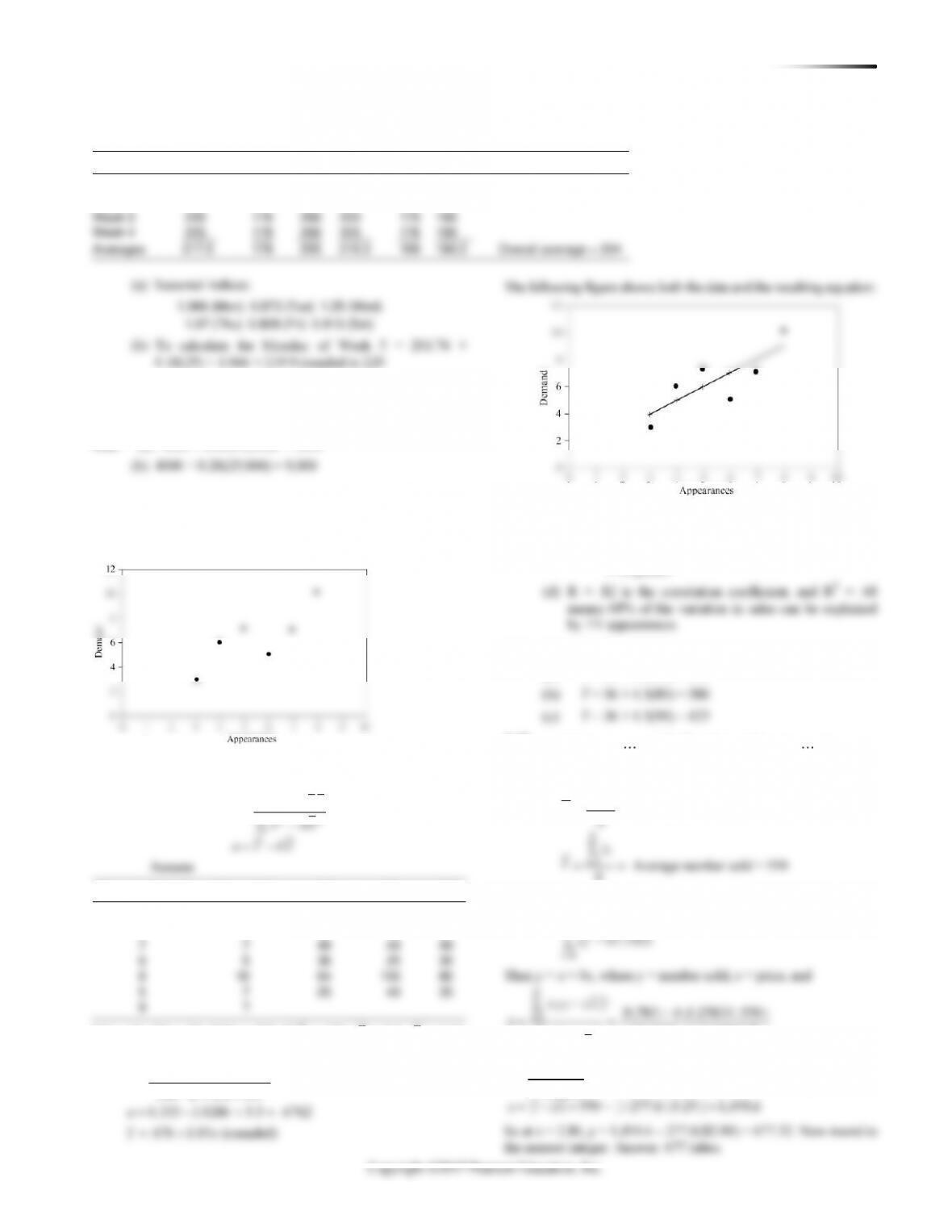
4.43 (a) Graph of demand
The observations obviously do not form a straight line but do tend
to cluster about a straight line over the range shown.
(b) Least-squares regression:
22
Y a bX
XY nXY
b
X nX
a Y bX
=+
−
=−
=−
Appearances X
Demand Y
X2
Y2
XY
3
3
9
9
9
4
6
16
36
24
7
7
49
49
49
6
5
36
25
30
8
10
64
100
80
5
7
25
49
35
9
?
X = 33, Y = 38, XY = 227, X2 = 199,
X
= 5.5,
Y
= 6.33.
Therefore:
b
==
227 – 6 5.5 6.333 1.0286
Week 4
225
178
260
225
176
190
(c) If there are nine performances by Maroon 5, the
estimated sales are:
9.676 1.03 9 .676 9.27 9.93 guitars
10 guitars
= + = + =
Y
4.44 Given Y = 36 + 4.3X
(a) Y = 36 + 4.3(70) = 337
4.45
=
=
=
=
==
=
1 2 6 1 2 6
6
1
6
1
6
1
62
1
Let , , , be the prices and , , ,
be the number sold.
Average price = 3.2583
6
6
9,783
= 67.1925
i
i
i
i
ii
i
i
i
x x x y y y
x
X
y
xy
x
Then y = a + bx, where y = number sold, x = price, and
6
1
62
22
1
9 783 6 3 25833 550
67 1925 6 3 25833
969 489 277 6
( , ) ( . )( )
. ( . )
..
ii
i
i
i
x y nxy
b
x nx
=
=
−
−
==
−
−
−
= = −
Mon.
Tue.
Wed.
Thu.
Fri.
Sat.
Week 1
210
178
250
215
160
180
Week 2
215
180
250
213
165
185
Week 3
220
176
260
220
175
190