12
C H A P T E R
Inventory Management
DISCUSSION QUESTIONS
1. The four types of inventory are:
been transferred
2. The advent of low-cost computing should not be seen as
Business organizations still have many items for which the cost of
LO 12.1: Conduct an ABC analysis
AACSB: Reflective thinking
LO 12.1: Conduct an ABC analysis
AACSB: Reflective thinking
4. Types of costs—holding cost: the cost of capital invested and
space required; shortage cost: the cost of lost sales or customers
who never return; the cost of lost goodwill; ordering cost: the
ble costs are the costs of placing an order or setting up production
and the cost of holding or storing inventory over time; and, if
orders are placed at the right time, stockouts or shortages can be
completely avoided.
LO 12.3: Explain and use the EOQ model for independent inven-
6. The EOQ increases as demand increases or as the setup cost
increases; it decreases as the holding cost increases. The changes
in the EOQ are proportional to the square root of the changes in
AACSB: Analytical thinking
quantity.
8. Advantages of cycle counting:
2. Eliminating annual inventory adjustments
3. Providing trained personnel to audit the accuracy of
inventory
5. Maintaining accurate inventory records
LO 12.2: Explain and use cycle counting
AACSB: Reflective thinking
9. A decrease in setup time decreases the cost per order,
encourages more and smaller orders, and thus decreases the EOQ.
point above the EOQ.)
LO 12.6: Explain and use the quantity discount model
AACSB: Analytical thinking
11. Service level refers to the probability that demand will not
186 CHAPTER 12 IN V E N TO R Y MA N A G E M E N T
END–OF-CHAPTER PROBLEMS (PROBLEMS WITH
12.1 An ABC system generally classifies the top 70% of dollar
volume items as A, the next 20% as B, and the remaining 10% as
C items. Similarly, A items generally constitute 20% of total
12.2 (a) You decide that the top 20% of the 10 items, based on a
value, but in larger samples the value would probably approach
70% to 80%.) You therefore rate items F3 and G2 as A items. The
next 30% of the items are A2, C7, and D1; they represent 25.5%
CHAPTER 12 IN V E N T O RY MA N A G E M E N T 187
12.4
7,000 0.10 = 700
700 20 = 35
35 A items per day
7,000 0.35 = 2,450
2450 60 = 40.83
41 B items per day
7,000 0.55 = 3,850
3850 120 = 32
12.5*
Annual
SKU
Demand
Cost ($)
Demand Cost
Classification
E
150
75
11,250
B
12.6*
Annual
Demand
Item
Demand
Cost ($)
Cost
Classification
E102
800
4.00
3,200
C
D23
1,200
8.00
9,600
A
27%
D27
700
3.00
2,100
C
R02
1,000
2.00
2,000
C
R19
200
8.00
1,600
C
S107
500
6.00
3,000
C
S123
1,200
1.00
1,200
C
U11
800
7.00
5,600
B
16%
U23
1,500
1.00
1,500
C
33%
12.7 (a)
2(19,500)(25)
EOQ = 493.71 494 units
4
Q= = =
12.8 (a)
==
2(8,000)(45)
EOQ 600 units
2
12.10 (a) Economic Order Quantity (Holding cost = $5 per year):
2 2 400 40 80 units
DS
holding cost
(b) Economic Order Quantity (Holding cost = $6 per year):
2 2 400 40 73 units
DS
12.11 D = 15,000, H = $25/unit/year, S = $75
25
H
(b) Annual holding costs = (Q/2) H = (300/2)
25 = $3,750
300 days
12.12 (a) Reorder point = Demand during lead time
ROP = [Demand/Day](Lead time) =
(c) If demand during lead time drops to 50 units/day,
ROP = 50 units/day × 21 days = 1,050 units.
12.13 (a) D = 10,000
ROP = [Demand/Day](Lead time) = [10,000/300](5)
= 166.67 167 units.
188 CHAPTER 12 IN V E N TO R Y MA N A G E M E N T
(b)
250
Average inventory 125 units
22
Q
= = =
Annual holding cost 125(1.50) $187.50
2
QH= = =
2500
D
Annual order cost 10(18.75) $187.50
DS
Q
= = =
(d)
TC 187.50 187.50 $375/ year
2
QD
HS
Q
= + = + =
Working days
would have to be for the order policy of 150 units to
be optimal. To find the answer to this problem, we
must solve the traditional economic order quantity
equation for the ordering (setup) cost. As you can see
in the calculations that follow, an ordering (setup)
DS
QH
H
SQ D
=
=
2
2
2
2
CHAPTER 12 IN V E N T O RY MA N A G E M E N T 189
2 2(12,000)50
40
DS
Q
d
==
= 4,472 lights per run
QdH
12.22 D (Annual demand) = 400 12 = 4,800, P (Purchase
price/Unit) = $350/unit, H (Holding cost /Unit) = $35/unit/year,
(a)
DS
QH
2 2 × 4, 800 ×120
== 35
190 CHAPTER 12 IN V E N TO R Y MA N A G E M E N T
Because 30 < 300, this EOQ is infeasible for the $380 price. So
Step 2 uses (12-9) to compute the total cost of the candidate order
CHAPTER 12 IN V E N T O RY MA N A G E M E N T 191
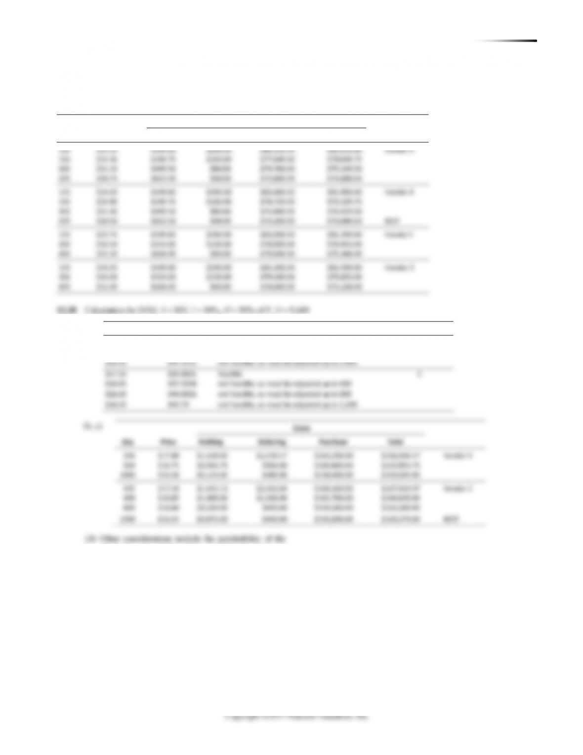
12.27 S = 10, H = 3.33, D = 2,400
120
Vendor A
150
300
120
Vendor B
150
300
120
Vendor C
200
120
Vendor D
200
$17.10
335.0831
feasible
2
$16.85
337.5598
not feasible, so must be adjusted up to 400
Vendor 1
Vendor 2
chemical and whether there is adequate space in
the controlled environment to handle 1,200 pounds of
the chemical at one time.
EOQ = 120 with slight rounding
Costs
Qty
Price
Holding
Ordering
Purchase
Total
(a)
Price
EOQ
Vendor
$17.00
336.0672
feasible
1
$16.75
338.5659
not feasible, so must be adjusted up to 500