trimmed multiple regression. Continue until only statistically significant betas are
left.
8. Using the bicycle example in question 7, what do you expect would be the elimination
of variables sequence using stepwise multiple regression? Explain your reasoning
with respect to the operation of this technique.
With stepwise regression, the first independent variable to be included is the one that
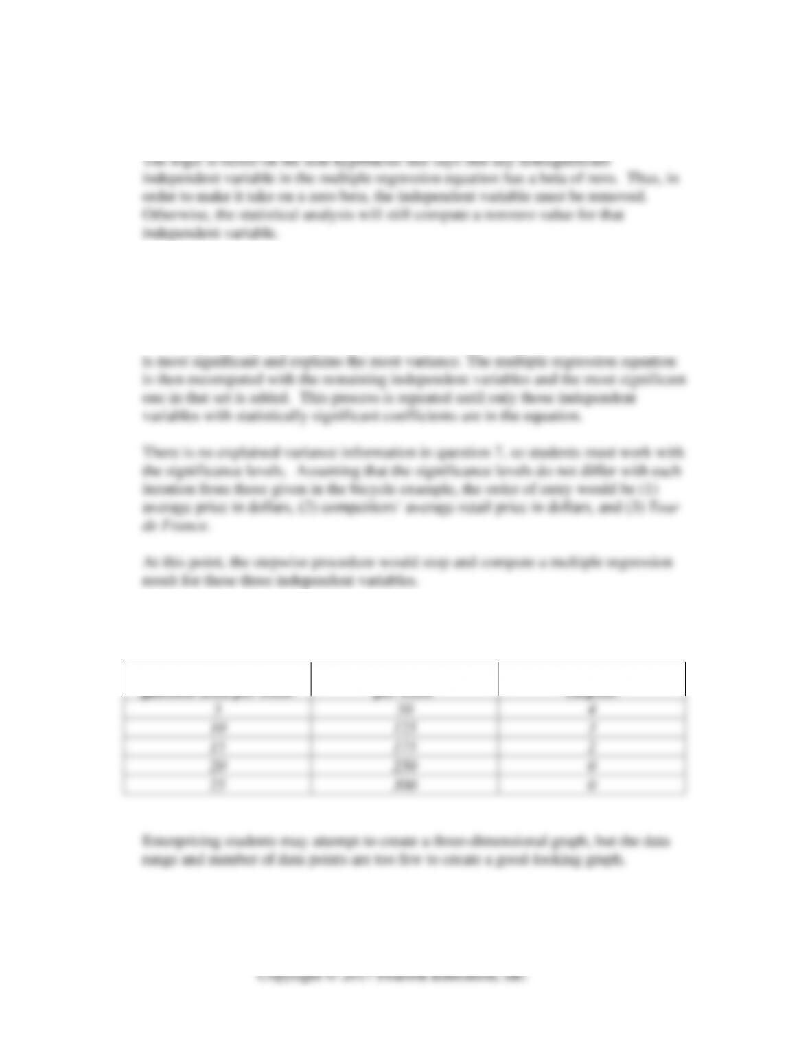
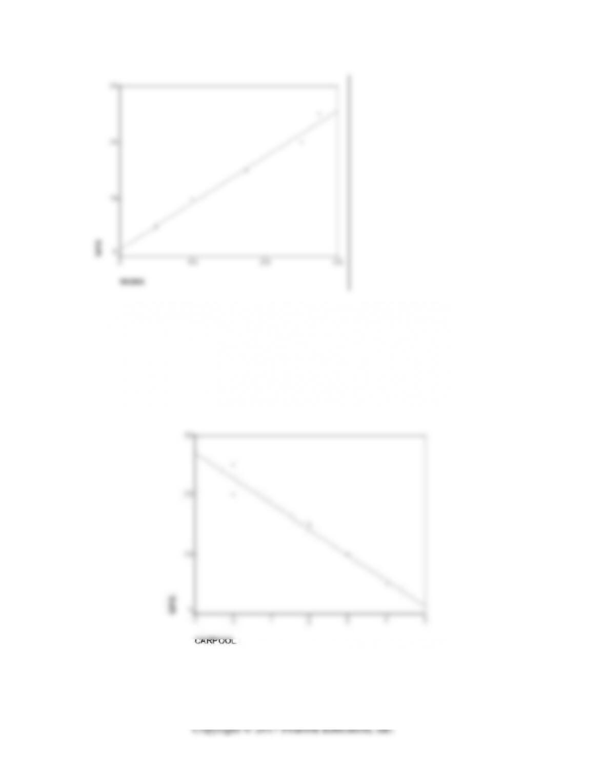
9. Using SPSS graphical capabilities, diagram the regression plane for the following
variables.
Number of gallons of
gasoline used per week
Miles commuted to work
per week
Number of riders in
carpool
5
50
4
10
125
3
15
175
2
20
250
0
25
300
0
Enterprising students may attempt to create a three-dimensional graph, but the data
range and number of data points are too few to create a good-looking graph.
10. The Maximum Amount is a company that specializes in making fashionable clothes in
large sizes for plus-sized people. A survey was performed for the Maximum Amount,
and a regression analysis was run on some of the data. Of interest in this analysis
was the possible relationship self-esteem (dependent variable) and number of
Maximum Amount articles purchased last year (independent variable). Self-esteem
was measured on a 7-point scale where 1 signifies very low and 7 indicates very high
self-esteem. Following are some items that have been taken from the output.
Pearson product moment correlation = +0.63
Intercept = 3.5
Slope = +0.2
All statistical tests are significant at the .01 level or less. What is the correct
interpretation of these findings?
11. Wayne LaTorte is a safety engineer who works for the U.S. Postal Service. For most
of his life, Wayne has been fascinated by UFOs. He has kept records of UFO
sightings in the desert areas of Arizona, California, and New Mexico over the past 15
years and he has correlated them with earthquake tremors. A fellow engineer
suggests that Wayne use regression analysis as a means of determining the
relationship. Wayne does this and finds a “constant” of 30 separate earth tremor
events and a slope of 5 events per UFO sighting. Wayne then writes an article for the
UFO Observer claiming that earthquakes are largely caused by the subsonic
vibrations emitted by UFOs as they enter the Earth’s atmosphere. What is your
reaction to Wayne’s article?
Can students spot this misuse of regression?
CASE SOLUTIONS
Case 15.1 L’Experience Félicité Restaurant Survey Predictive Analysis
Case Objective
Students must apply predictive analysis on L’Experience Félicité Restaurant survey SPSS
case data set and interpret the findings.
Answers to Case Questions
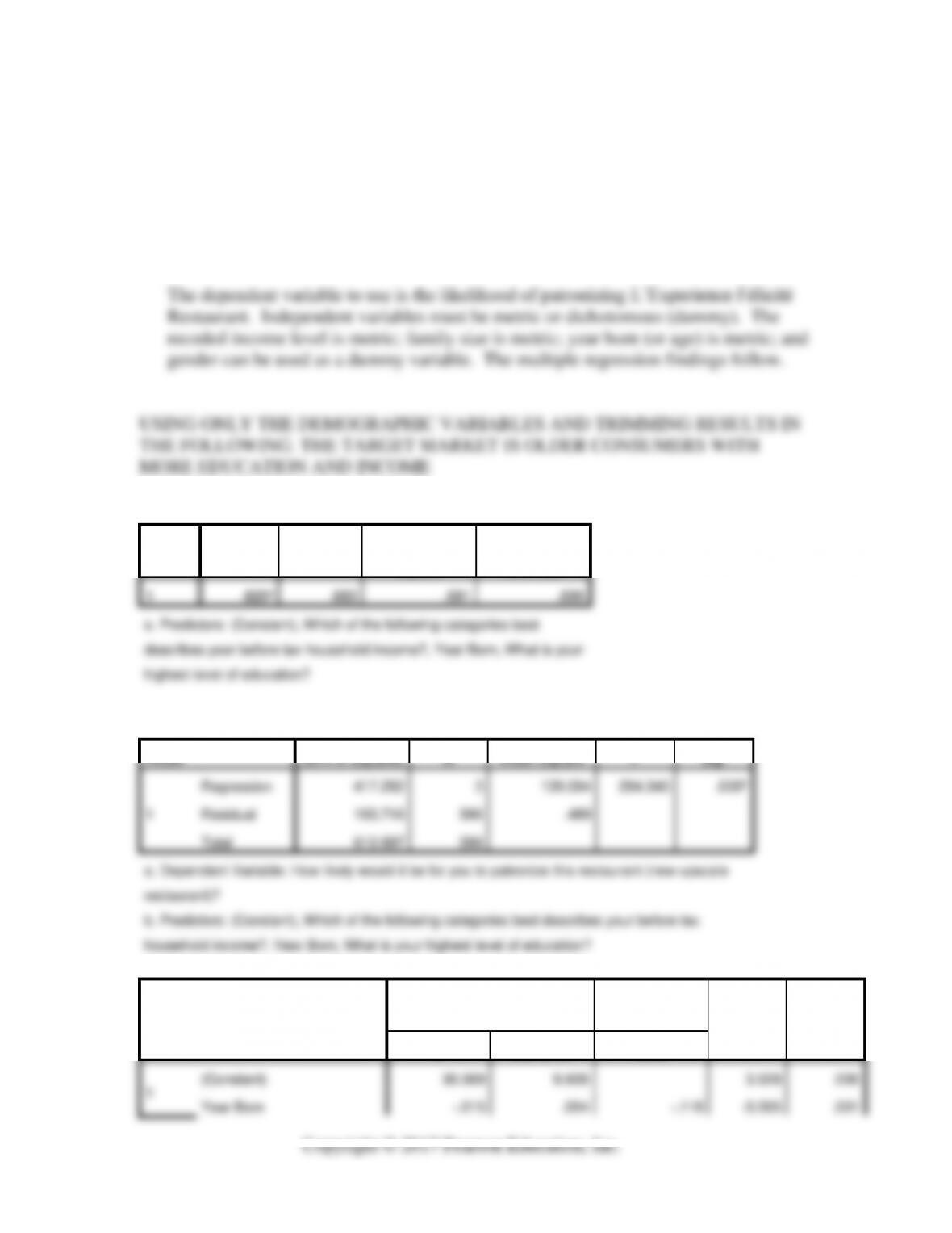
1. What is the demographic target market definition for L’Experience Félicité
Restaurant?
Model Summary
Model
R
R Square
Adjusted R
Square
Std. Error of the
Estimate
1
.826a
.683
.681
.699
a. Predictors: (Constant), Which of the following categories best
describes your before tax household income?, Year Born, What is your
highest level of education?
ANOVAa
Model
Sum of Squares
df
Mean Square
F
Sig.
1
Regression
417.282
3
139.094
284.340
.000b
Residual
193.716
396
.489
Total
610.997
399
a. Dependent Variable: How likely would it be for you to patronize this restaurant (new upscale
restaurant)?
b. Predictors: (Constant), Which of the following categories best describes your before tax
household income?, Year Born, What is your highest level of education?
Coefficientsa
Model
Unstandardized Coefficients
Standardized
Coefficients
t
Sig.
B
Std. Error
Beta
1
(Constant)
30.369
8.608
3.528
.000
Year Born
-.015
.004
-.118
-3.505
.001
What is your highest level of
education?
.147
.033
.168
4.424
.000
Which of the following
categories best describes
your before tax household
income?
.470
.030
.664
15.833
.000
a. Dependent Variable: How likely would it be for you to patronize this restaurant (new upscale restaurant)?
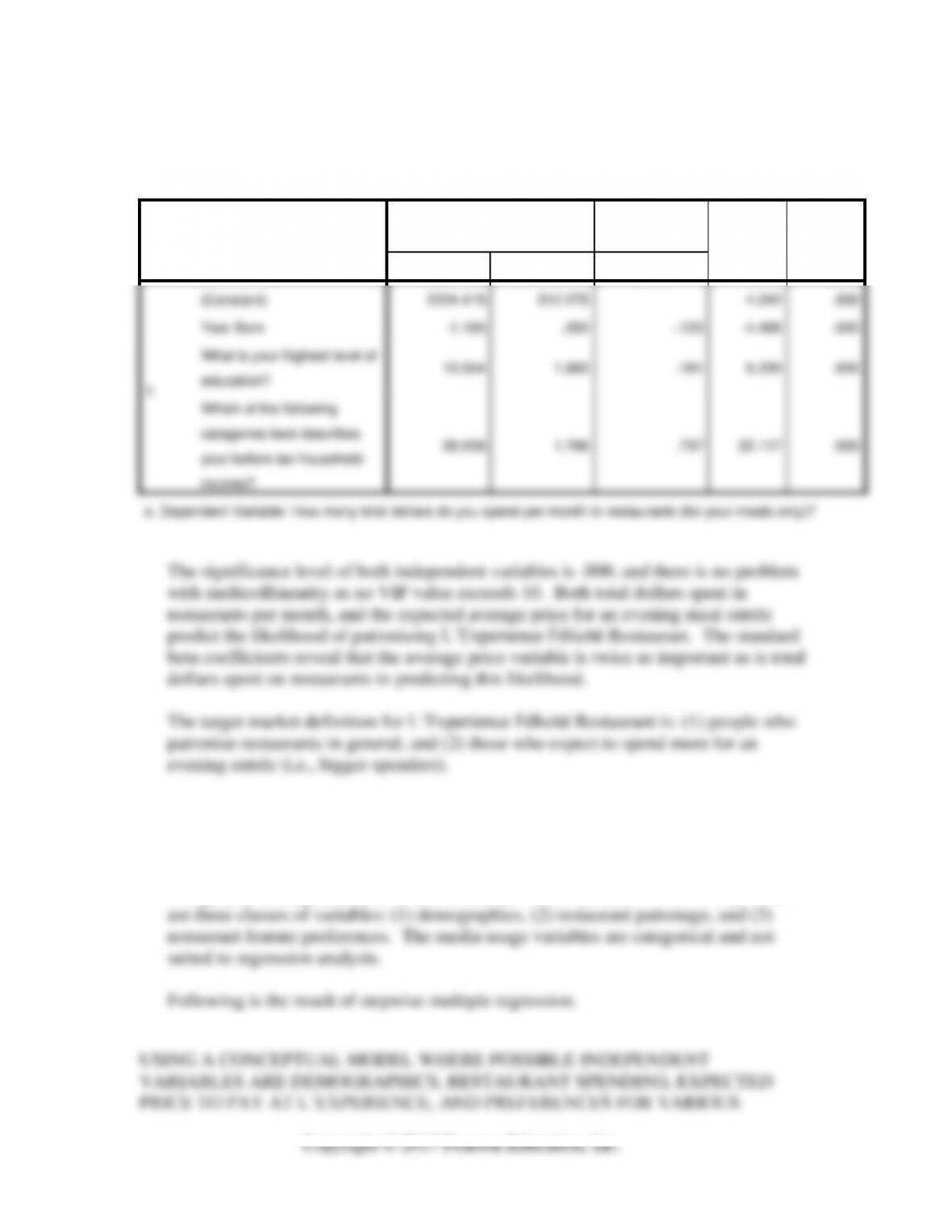
2. What is the restaurant spending behavior target market definition for L’Experience
Félicité Restaurant?
Model Summary
Model
R
R Square
Adjusted R
Square
Std. Error of the
Estimate
1
.894a
.800
.798
$41.62388
a. Predictors: (Constant), Which of the following categories best
describes your before tax household income?, Year Born, What is your
highest level of education?
ANOVAa
Model
Sum of Squares
df
Mean Square
F
Sig.
1
Regression
2743099.063
3
914366.354
527.758
.000b
Residual
686088.835
396
1732.548
Total
3429187.897
399
a. Dependent Variable: How many total dollars do you spend per month in restaurants (for your
meals only)?
b. Predictors: (Constant), Which of the following categories best describes your before tax
household income?, Year Born, What is your highest level of education?
Coefficientsa
Model
Unstandardized Coefficients
Standardized
Coefficients
t
Sig.
B
Std. Error
Beta
1
(Constant)
2224.415
512.275
4.342
.000
Year Born
-1.165
.260
-.120
-4.486
.000
What is your highest level of
education?
10.554
1.980
.161
5.330
.000
Which of the following
categories best describes
your before tax household
income?
39.056
1.766
.737
22.117
.000
a. Dependent Variable: How many total dollars do you spend per month in restaurants (for your meals only)?
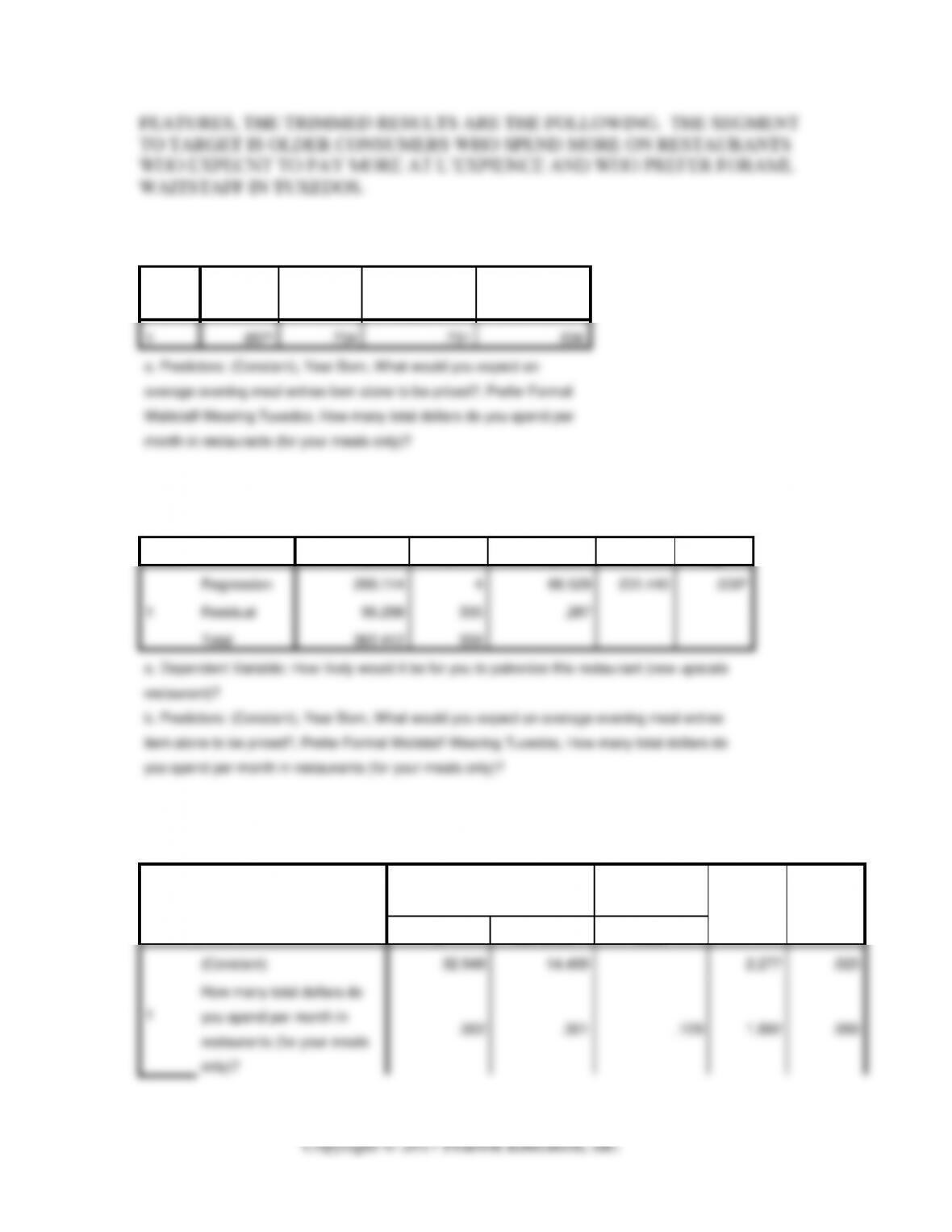
3. Develop a general conceptual model of market segmentation for L’Experience
Félicité Restaurant. Test it using multiple regression analysis and interpret your
findings for Jeff Dean.
The general conceptual model should be based on the variables in the survey. There
Model Summary
Model
R
R Square
Adjusted R
Square
Std. Error of the
Estimate
1
.857a
.734
.731
.536
a. Predictors: (Constant), Year Born, What would you expect an
average evening meal entree item alone to be priced?, Prefer Formal
Waitstaff Wearing Tuxedos, How many total dollars do you spend per
month in restaurants (for your meals only)?
ANOVAa
Model
Sum of Squares
df
Mean Square
F
Sig.
1
Regression
266.114
4
66.529
231.440
.000b
Residual
96.298
335
.287
Total
362.412
339
a. Dependent Variable: How likely would it be for you to patronize this restaurant (new upscale
restaurant)?
b. Predictors: (Constant), Year Born, What would you expect an average evening meal entree
item alone to be priced?, Prefer Formal Waitstaff Wearing Tuxedos, How many total dollars do
you spend per month in restaurants (for your meals only)?
Coefficientsa
Model
Unstandardized Coefficients
Standardized
Coefficients
t
Sig.
B
Std. Error
Beta
1
(Constant)
32.948
14.469
2.277
.023
How many total dollars do
you spend per month in
restaurants (for your meals
only)?
.002
.001
.129
1.892
.059
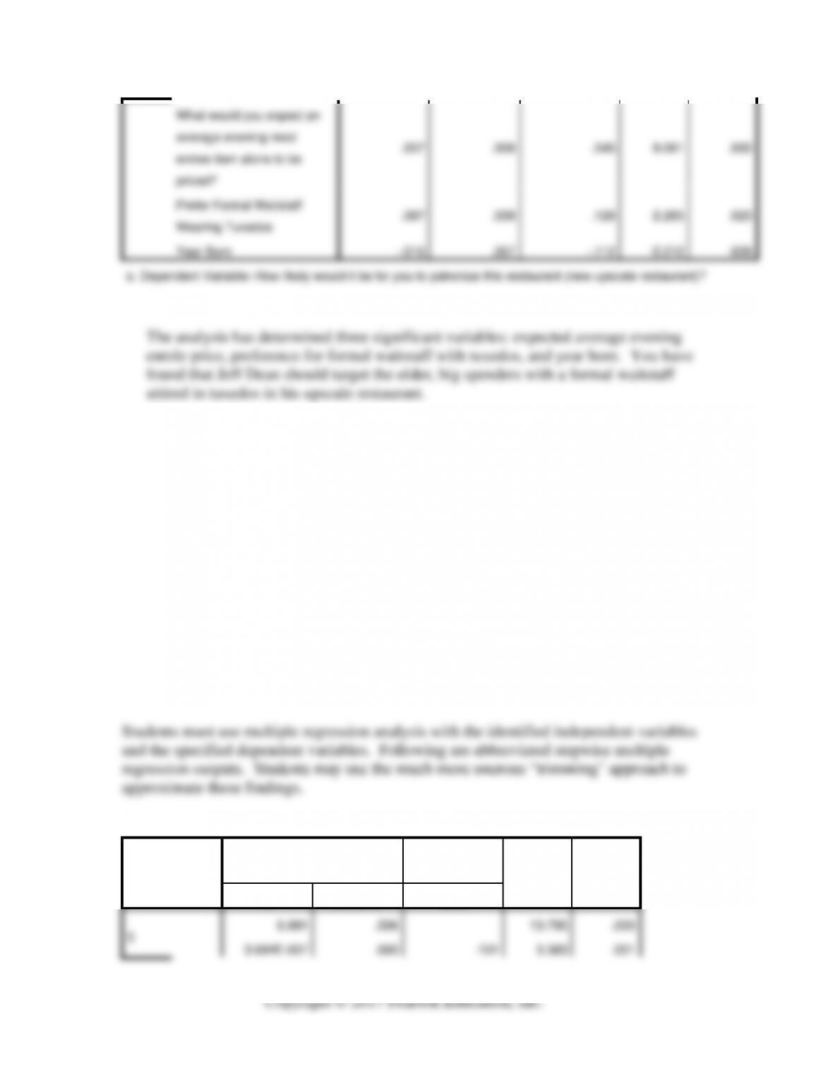
What would you expect an
average evening meal
entree item alone to be
priced?
.057
.006
.545
9.061
.000
Prefer Formal Waitstaff
Wearing Tuxedos
.087
.038
.128
2.283
.023
Year Born
-.016
.007
-.112
-2.212
.028
a. Dependent Variable: How likely would it be for you to patronize this restaurant (new upscale restaurant)?
Case 15.2 Auto Concepts Segmentation Analysis
Case Objective
Answers to Case Questions
With each hybrid automobile model, prepare a summary that does the following:
1. Lists the statistically significant independent variables (use 95% level of confidence).
2. Interprets the directional of the relationship of each statistically significant
independent variable with respect to the preference for the hybrid model concerned.
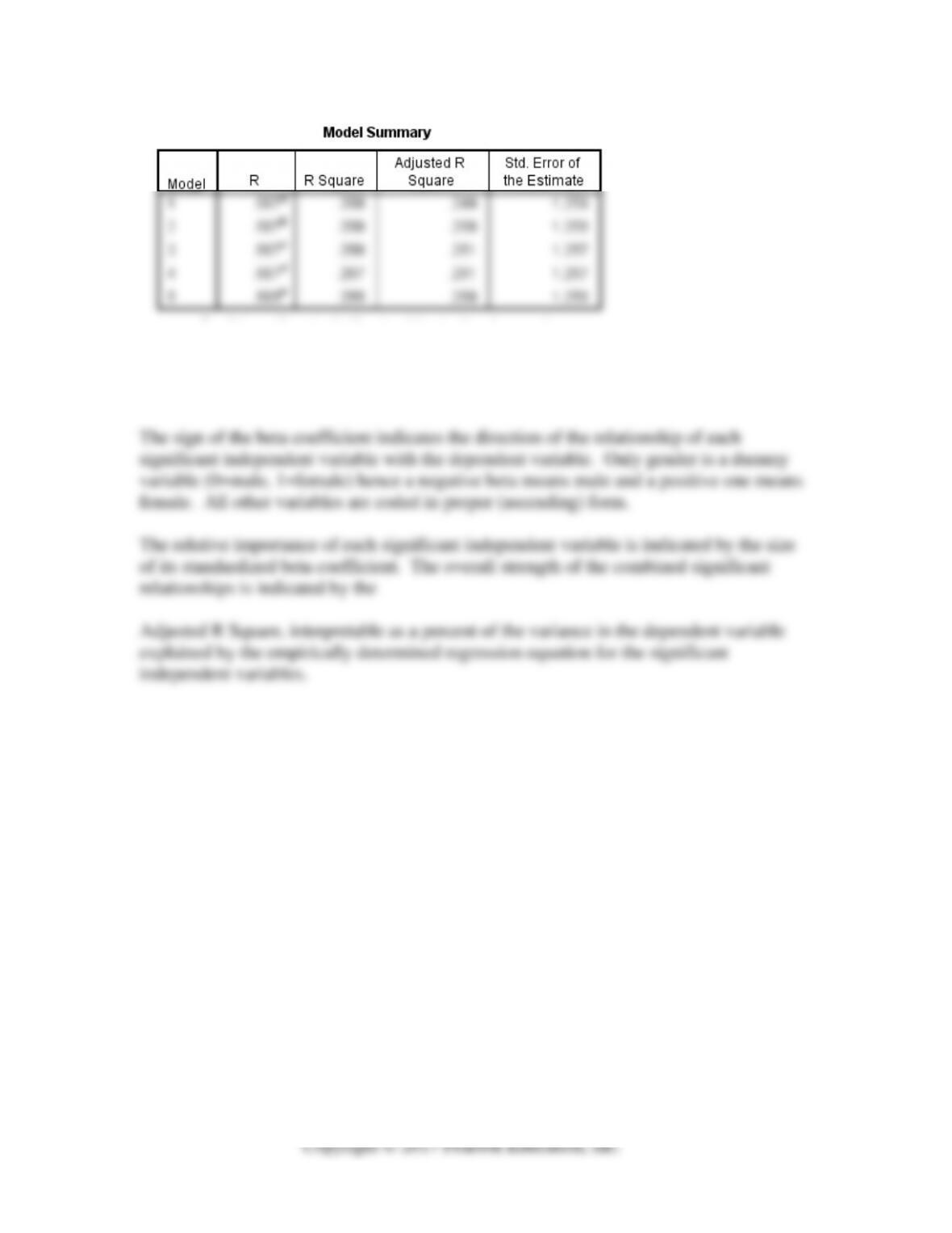
3. Identifies or distinguishes the relative importance of each of the statistically significant
independent variables.
4. Assesses the strength of the statistically significant independent variables as they join
to predict the preferences for the hybrid model concerned.
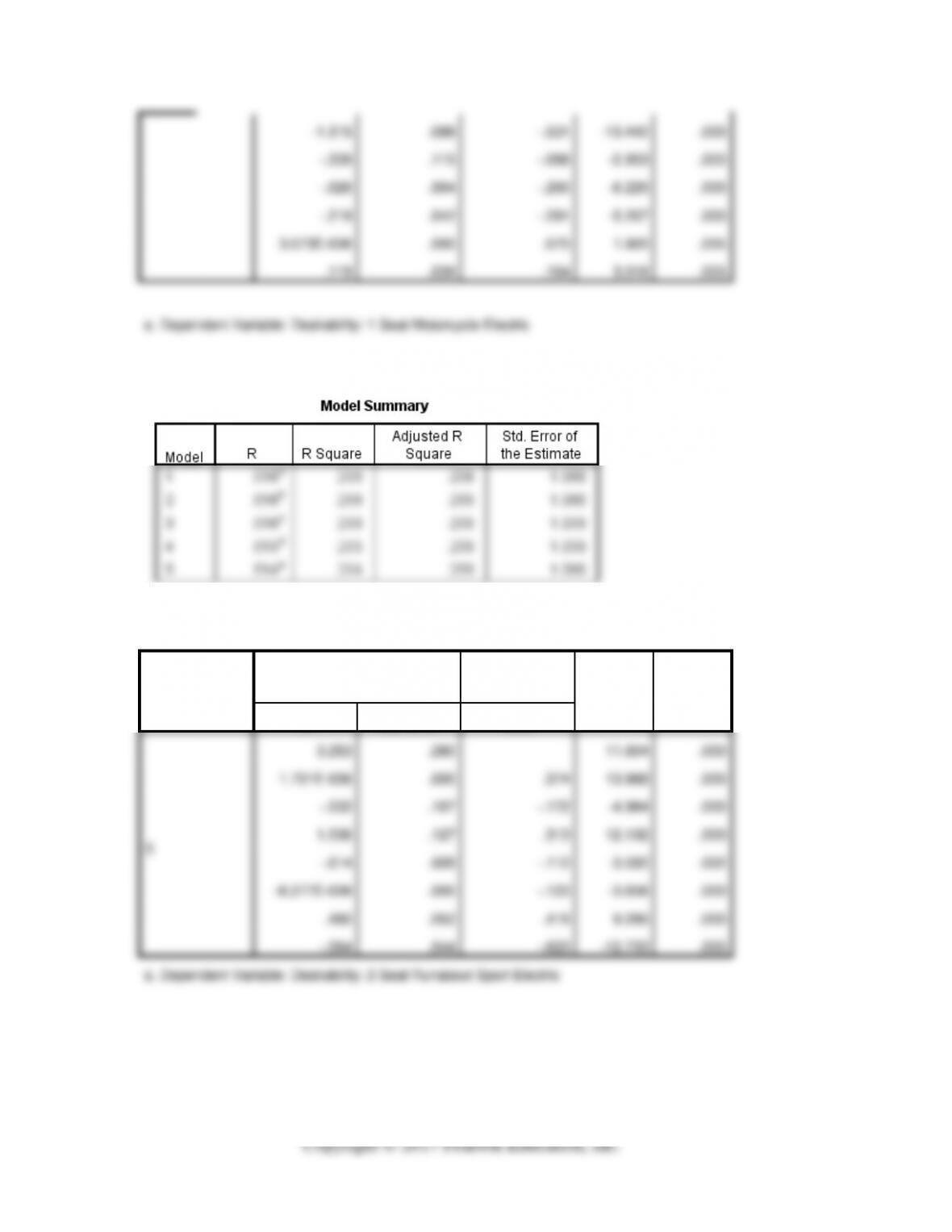
Coefficientsa
Model
Unstandardized Coefficients
Standardized
Coefficients
t
Sig.
B
Std. Error
Beta
5
6.981
.506
13.795
.000
3.694E-007
.000
.101
3.383
.001
-1.315
.098
-.531
-13.442
.000
-.339
.115
-.086
-2.953
.003
-.026
.004
-.260
-6.220
.000
-.219
.042
-.291
-5.207
.000
3.073E-006
.000
.075
1.920
.055
.119
.039
.164
3.016
.003
a. Dependent Variable: Desirability: 1 Seat Motorcycle Electric
Coefficientsa
Model
Unstandardized Coefficients
Standardized
Coefficients
t
Sig.
B
Std. Error
Beta
5
3.253
.280
11.604
.000
1.701E-006
.000
.374
13.988
.000
-.532
.107
-.172
-4.984
.000
1.536
.127
.313
12.132
.000
-.014
.005
-.112
-3.032
.002
-6.277E-006
.000
-.123
-3.656
.000
.480
.052
.415
9.295
.000
-.564
.044
-.623
-12.733
.000
a. Dependent Variable: Desirability: 2 Seat Runabout Sport Electric
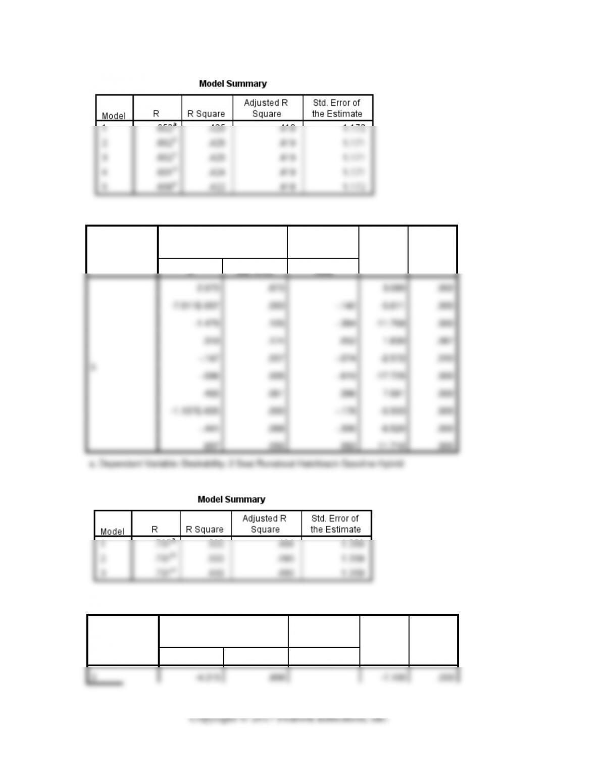
Model
Unstandardized Coefficients
Standardized
Coefficients
t
Sig.
B
Std. Error
Beta
3
2.073
.673
3.080
.002
-7.911E-007
.000
-.140
-5.611
.000
-1.479
.126
-.384
-11.768
.000
.318
.174
.052
1.830
.067
-.147
.057
-.074
-2.572
.010
-.096
.005
-.619
-17.725
.000
.465
.061
.396
7.591
.000
-1.137E-005
.000
-.178
-5.503
.000
-.441
.068
-.306
-6.520
.000
.657
.056
.583
11.710
.000
a. Dependent Variable: Desirability: 2 Seat Runabout Hatchback Gasoline Hybrid
Coefficientsa
Model
Unstandardized Coefficients
Standardized
Coefficients
t
Sig.
B
Std. Error
Beta
3
-4.315
.608
-7.100
.000
1.476E-006
.000
.282
11.371
.000
.469
.116
.132
4.037
.000
-.440
.161
-.078
-2.742
.006
.220
.053
.119
4.145
.000
.056
.005
.391
11.244
.000
.151
.052
.139
2.893
.004
1.991E–005
.000
.338
10.459
.000
.182
.048
.175
3.809
.000
-.086
.036
-.074
-2.385
.017
a. Dependent Variable: Desirability: 4 Seat Economy Diesel Hybrid
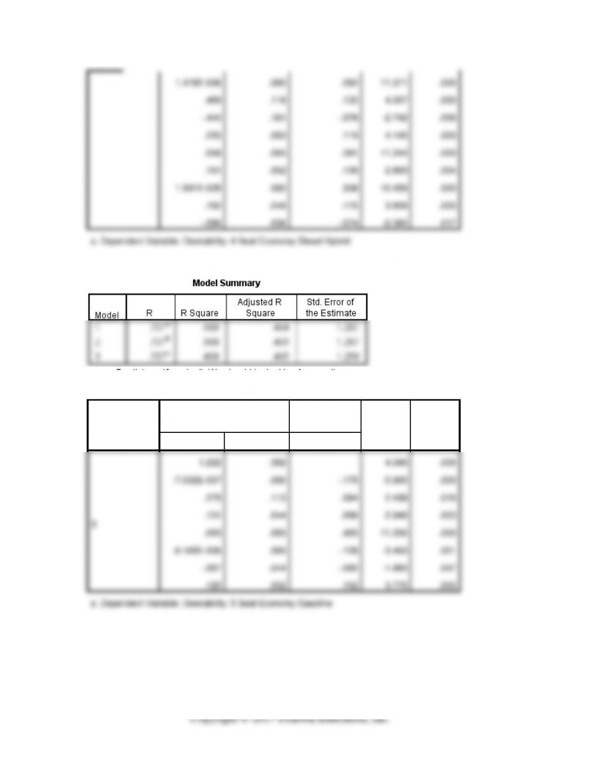
Coefficientsa
Model
Unstandardized Coefficients
Standardized
Coefficients
t
Sig.
B
Std. Error
Beta
5
1.222
.302
4.049
.000
-7.532E-007
.000
-.175
-5.905
.000
.275
.113
.094
2.439
.015
.131
.044
.086
2.948
.003
.055
.005
.465
11.050
.000
-6.185E-006
.000
-.128
-3.463
.001
-.087
.044
-.080
-1.993
.047
.120
.032
.152
3.770
.000
a. Dependent Variable: Desirability: 5 Seat Economy Gasoline
Statistically significant variables as those with Sig. <=.05.