
CHAPTER 14
MAKING USE OF ASSOCIATIONS TESTS
LEARNING OBJECTIVES
In this chapter you will learn:
14-1 The types of relationships between two variables
14-2 How relationships between two variables may be characterized
14-3 What correlation coefficients and covariation are
14-4 About the Pearson Product Moment Correlation Coefficient and how to obtain in
with SPSS
14-5 The way to report correlation findings to clients
14-6 What cross-tabulations are and how to compute them
14-7 Chi-square analysis and how it is used in cross-tabulation analysis
14-8 The way to report cross-tabulation findings to clients
14-9 Special considerations when performing association analyses such as correlations
and cross-tabulations
CHAPTER OUTLINE
Types of Relationships Between Two Variables
• Linear and Curvilinear Relationships
• Monotonic Relationships
• Nonmonotonic Relationships
Characterizing Relationships Between Variables
• Presence
• Direction (or Pattern)
• Strength of Association
Correlation Coefficients and Covariation
Copyright © 2017 Pearson Education, Inc.
• Rules of Thumb for Correlation Strength
• The Correlation Sign: The Direction of the Relationship
• Graphing Covariation Using Scatter Diagrams
The Pearson Product Moment Correlation Coefficient
Reporting Correlation Findings to Clients
Cross-Tabulations
• Cross-Tabulation Analysis
• Types of Frequencies and Percentages in a Cross-Tabulation Table
Chi-Square Analysis
• Observed and Expected Frequencies
• The Computed χ² Value
• The Chi-Square Distribution
• How to Interpret a Chi-Square Result
Reporting Cross-Tabulation Findings to Clients
Special Considerations in Association Procedures
KEY TERMS
Associative analyses Relationship
Nonmonotonic relationship Monotonic relationships
Linear relationship Straight-line formula
Curvilinear relationship Cross-tabulation table
Cross-tabulation cell Frequencies table
Raw percentages table Column percentages table
Row percentages table Chi-square (
2
) analysis
Observed frequencies Expected frequencies
Chi-square formula Chi-square distribution
Correlation coefficient Covariation

Scatter diagram Pearson product moment correlation
Cause and effect relationship
TEACHING SUGGESTIONS
1. The reason for describing the various types of relationships possible between
variables is to bridge the scaling assumptions of variables and the appropriate
statistical analysis. Students should come away from this section of the chapter with
the following understanding: The crudest scales (i.e., nonmonotonic which are merely
categories with no order or magnitude) necessitate the use of chi-square analysis
predicated on cross-tabulations. Ordinal scales effect order in the categories, but
there is no indication of distances in magnitude among adjacent categories, so two
ordinal scaled variables can be examined for a monotonic relationship with rank order
correlation. Interval and ratio scales embody order and specific units of distance
among the categories. The precise measurements of two “metric” scaled variables
allows use of a linear relationship which is the underlying basis for Pearson Product
Moment correlation.
2. Instructors may want to provide examples of how higher scaled variables can be
“collapsed down” to lower scaled ones. For instance, age in years (ratio) can be
collapsed to ordinal by setting up arbitrary categories of “youth,” “young adult,”
“middle–aged adult,” “old adult,” and “elderly.” Similarly, an ordinal scaled variable
can be collapsed to a nominal one with a median split, classifying respondents as
either “high” or “low.”
Collapsing variables to be measured on lower level scales is useful in the following
circumstances.
a. When you want to investigate a relationship between variables with different
scaling assumptions. For example, income measured as ordinal can be collapsed
down to nominal to look at the relationship of income to user type (user versus
nonuser) which is nominal.
b. When higher level scaled variables exhibit no statistically significant relationship,

d. When sample sizes are very small, collapsing will increase the size of the scale
category subsample. For instance, if there are 30 respondents and 25 metric scale
categories (such as age in years), collapsing to a high-low designation using the
median will result in 15 high- and 15 low-age respondents.
3. SPSS cross-tabulations includes several nominal-to-nominal variable nonparametric
statistics options such as contingency coefficient, Phi, Lambda, and others. It also
4. The null hypothesis is omnipresent in associative analysis tests, and it is the
foundation for practically all statistical tests. Instructors are recommended to
continually remind students of the null hypothesis of no association as they review
the various associative analysis tests. It may be worthwhile to recall for students that
the null hypothesis is present in statistical inference tests such as t tests (no difference
between the means of the two groups) or analysis of variance (no difference between
any two group means). For instructors’ information, the null hypothesis concept is
emphasized in the next chapter, particularly with descriptions of bivariate and
multiple regression analyses.
5. Experience has taught that students will become confused with initial encounters with
the various types of frequencies and percentages possible in cross-tabulation tables.
The chapter takes students step-by-step through these slowly; however, Instructors
should consider using class time to review the various steps so students will gain a
conceptual understanding of what each type is and how it is used. At the very least,
students should understand how row and column percentages are useful in identifying
the underlying association if statistical significance is found.
For instructors who want their students to actually compute correlation statistics,
consider end-of-chapter question number 14. It has only 10 cases. The answer to
6. Instructors who desire to emphasize the scatter diagram interpretation of a correlation
should also consider using end-of-chapter question 14. The correlation matrix for all
five variables is provided following as are two scatter diagrams for extreme
correlations (high positive and essentially zero). Students should be able to build the
dataset in SPSS quickly, and they can have SPSS create all possible scatter diagrams.
7. Question 14 is also a useful in-class example. If one has SPSS capabilities in the
classroom, the scatter diagram interpretation of correlation can be illustrated quickly
and effectively using the small dataset provided in question 14.
ACTIVE LEARNING EXERCISES
Compute Chi-Square Values
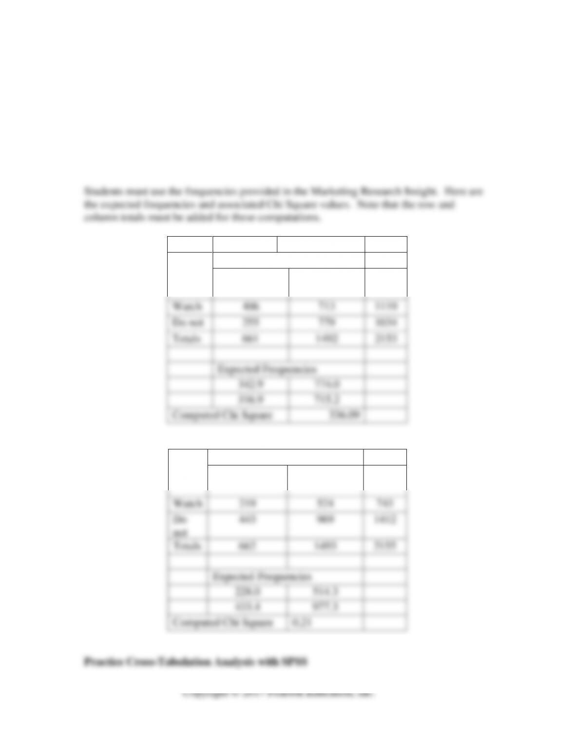
Marketing Research Insight 18.3 has a cross-tabulation for a sports marketing survey
that compared Generation X with Generation Y television viewers of professional sports.
Compute the expected frequencies and chi square values for each one.
NFL Games
Generation X
Generation Y
Totals
Watch
406
713
1119
Do not
255
779
1034
Totals
661
1492
2153
Expected Frequencies
342.9
774.0
316.9
715.2
Computed Chi Square
336.09
NBA Games
Generation X
Generation Y
Totals
Watch
219
524
743
Do
not
443
969
1412
Totals
662
1493
2155
Expected Frequencies
228.0
514.3
433.4
977.3
Computed Chi Square
0.21
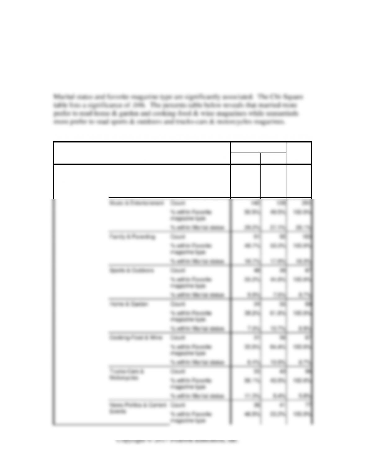
To make certain you can perform SPSS cross-tabulation with Chi-square analysis, use
the Auto Concepts SPSS data set and replicate the Gender–Favorite magazine type
analysis just described. When you are convinced that you can do this analysis correctly
and interpret the output, use it to see if there is an association between marital status and
favorite magazine type. What about marital status and newspaper reading habits?
Favorite magazine type * Marital status Crosstabulation
Marital status
Total
Unmarried
Married
Favorite magazine
type
Business & Money
Count
50
48
98
% within Favorite
magazine type
51.0%
49.0%
100.0%
% within Marital status
10.3%
9.4%
9.8%
Music & Entertainment
Count
142
139
281
% within Favorite
magazine type
50.5%
49.5%
100.0%
% within Marital status
29.2%
27.1%
28.1%
Family & Parenting
Count
91
92
183
% within Favorite
magazine type
49.7%
50.3%
100.0%
% within Marital status
18.7%
17.9%
18.3%
Sports & Outdoors
Count
48
39
87
% within Favorite
magazine type
55.2%
44.8%
100.0%
% within Marital status
9.9%
7.6%
8.7%
Home & Garden
Count
34
55
89
% within Favorite
magazine type
38.2%
61.8%
100.0%
% within Marital status
7.0%
10.7%
8.9%
Cooking-Food & Wine
Count
31
56
87
% within Favorite
magazine type
35.6%
64.4%
100.0%
% within Marital status
6.4%
10.9%
8.7%
Trucks-Cars &
Motorcycles
Count
55
43
98
% within Favorite
magazine type
56.1%
43.9%
100.0%
% within Marital status
11.3%
8.4%
9.8%
News-Politics & Current
Events
Count
36
41
77
% within Favorite
magazine type
46.8%
53.2%
100.0%
Count
25
24
49
% within Marital status
7.4%
8.0%
7.7%
Total
Count
487
513
1000
% within Favorite
magazine type
48.7%
51.3%
100.0%
% within Marital status
100.0%
100.0%
100.0%
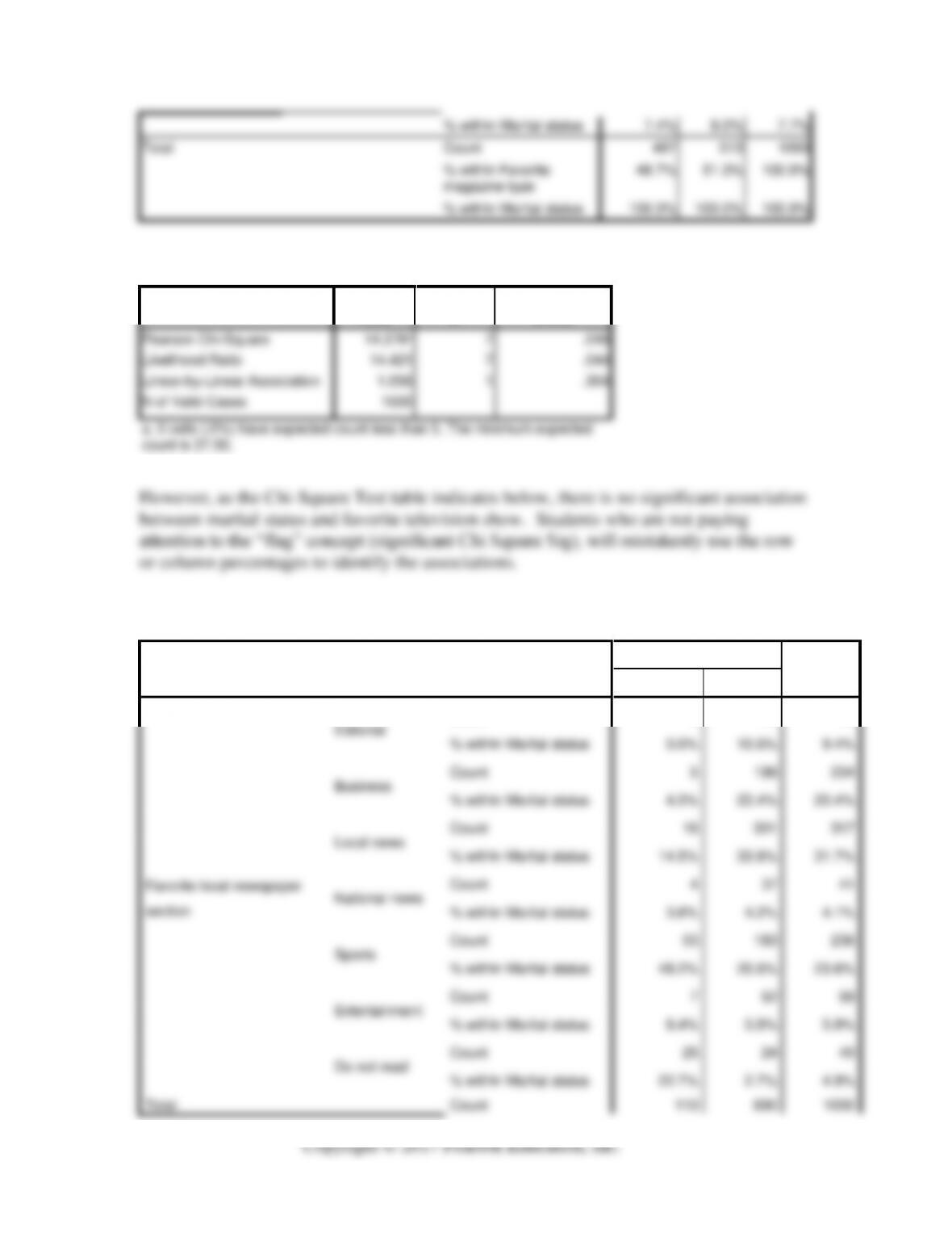
Chi-Square Tests
Value
df
Asymp. Sig. (2-
sided)
Pearson Chi-Square
14.276a
7
.046
Likelihood Ratio
14.421
7
.044
Linear–by-Linear Association
1.056
1
.304
N of Valid Cases
1000
a. 0 cells (.0%) have expected count less than 5. The minimum expected
count is 37.50.
Favorite local newspaper section * Marital status Crosstabulation
Marital status
Total
Unmarried
Married
Favorite local newspaper
section
Editorial
Count
0
94
94
% within Marital status
0.0%
10.6%
9.4%
Business
Count
5
199
204
% within Marital status
4.5%
22.4%
20.4%
Local news
Count
16
301
317
% within Marital status
14.5%
33.8%
31.7%
National news
Count
4
37
41
% within Marital status
3.6%
4.2%
4.1%
Sports
Count
53
183
236
% within Marital status
48.2%
20.6%
23.6%
Entertainment
Count
7
52
59
% within Marital status
6.4%
5.8%
5.9%
% within Marital status
100.0%
100.0%
100.0%
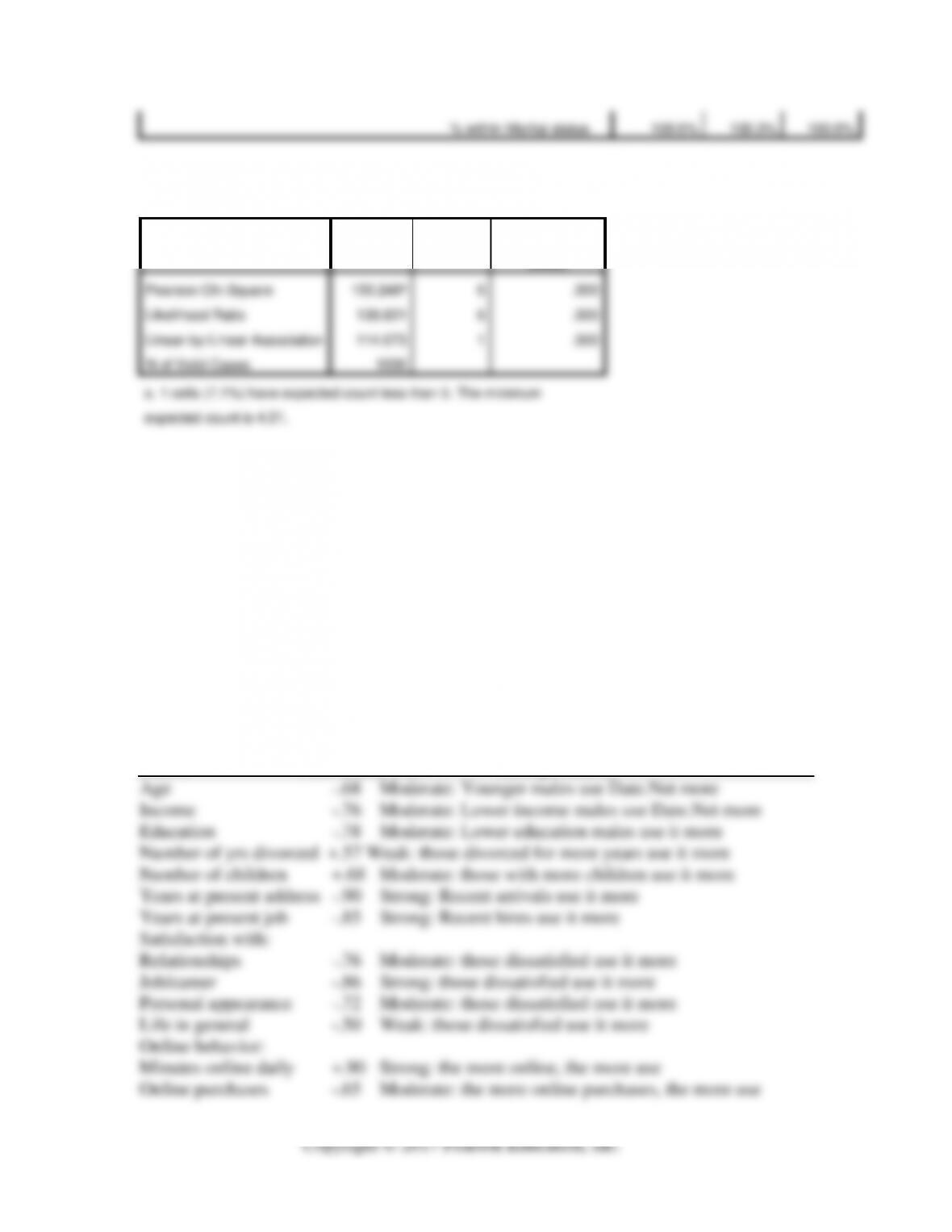
Chi-Square Tests
Value
df
Asymp. Sig. (2-
sided)
Pearson Chi-Square
150.240a
6
.000
Likelihood Ratio
130.821
6
.000
Linear–by-Linear Association
114.073
1
.000
N of Valid Cases
1000
a. 1 cells (7.1%) have expected count less than 5. The minimum
expected count is 4.51.
Date.net: Male Users’ Chat Room Phobia
For each factor, use your knowledge of correlations and provide a statement of how it
characterizes the typical Date.net male chat room user. Given your findings, what tactics
do you recommend to Date.net to address the low satisfaction with Date.net’s public chat
room that has been expressed by its female members?
The individual interpretations are in the table below. Students should realize that Date.net
needs to recruit a higher class of male users.
Correlation with
Amount of date.net
Factor Chat Room Use Interpretation

ANSWERS TO END-OF-CHAPTER QUESTIONS
1. Explain the distinction between a statistical relationship and a causal relationship.
2. Define and provide an example for each of the following types of relationship:
The definition and an example follow each type.
a. Linear
A linear relationship is a “straight–line association” between two variables. Here,
knowledge of the amount of one variable will automatically yield knowledge of the
b. Curvilinear

c. Nonmonotonic
d. Monotonic
Monotonic relationships are ones in which the researcher can assign only a general
3. Relate the three different aspects of a relationship between two variables.
Depending on the type, a relationship can be characterized in three ways: presence,
4. List the recommended steps for analyzing relationships.
Step 1: Choose variables to analyze.

5. Briefly describe the connections among the following: covariation, scatter diagram,
correlation, and linear relationship.
6. Indicate, with the use of a scatter diagram, the general shape of the scatter of data
points in each of the following cases:
The shapes are described after each correlation type.
a. A strong positive correlation
b. A weak negative correlation
c. No correlation
d. A correlation of -.98
7. What is meant by the term “significant correlation”?
8. What are the scaling assumptions assumed by Pearson product moment correlation?
9. What is a cross-tabulation? Give an example.
10. With respect to Chi-square analysis, describe or identify each of the following:
Each item is identified next.
a. r x c table
b. Frequencies table
c. Observed frequencies
d. Expected frequencies
e. Chi-square distribution
f. Significant association
g. Scaling assumptions
h. Row percentages versus column percentages
The column percentages table divides the raw cell frequencies by their respective
raw column total frequency. The formula is as follows:
i. Degrees of freedom

11. Listed here are various factors that may have relationships that are interesting to
marketing managers. With each one, (1) identify the type of relationship, (2) indicate
its nature or direction, and (3) specify how knowledge of the relationship could help a
marketing manager in designing marketing strategy.
The relationship, direction, and implication are listed beneath each case.
a. The amount (number of minutes per day) of time spent reading certain sections of
the Sunday newspaper and age of the reader for a sporting goods retail store.
b. Subscription to the local television cable company versus online TV viewing and
household income (low or high) for a telemarketing service being used by a
public television broadcasting station soliciting funds.
c. Number of miles driven in company cars and need for service such as oil changes,
tune-ups, or filter changes for a quick auto service chain attempting to market
fleet discounts to companies.
d. Plans to take a five-day vacation to Jamaica and the exchange rate of the
Jamaican dollar to that of other countries for Sandals, an all-inclusive resort
located in Montego Bay.

e. Homeowners opting for do-it-yourself home repairs and state of the economy (for
example, a recession or a boom) for Ace Hardware stores.
12. Indicate the presence, nature, and strength of the relationship involving purchases of
intermediate automobiles and each of the following factors: (a) price, (b) fabric
versus leather interior, (c) exterior color, and (d) size of rebate.
a. Price
b. Fabric versus leather interior
c. Exterior color
d. Size of rebate

13. With each of the following examples, compose a reasonable statement of an
association you would expect to find existing between the factors involved, and
construct a stacked bar chart expressing that association.
a. Wearing braces to straighten teeth by children attending expensive private
schools versus those attending public schools
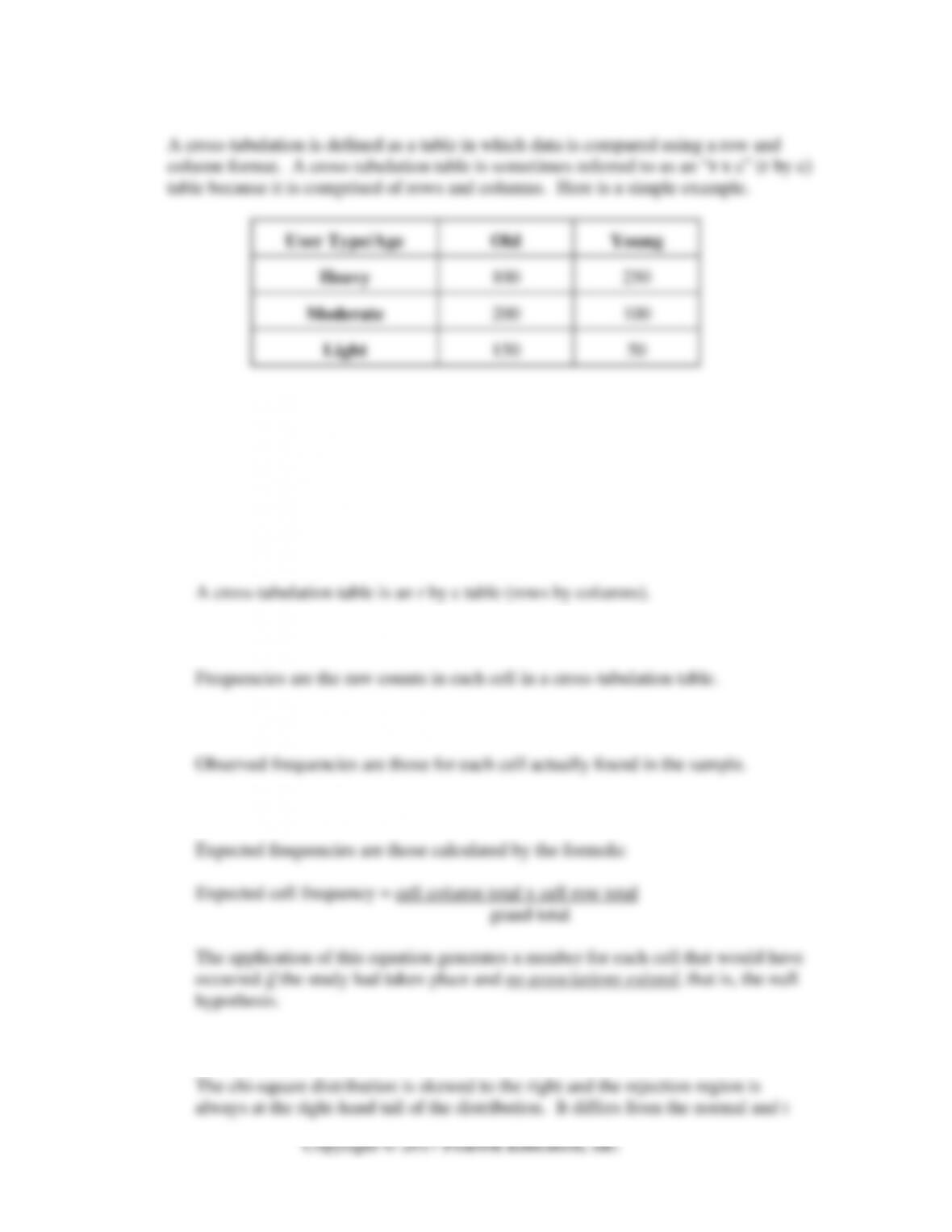
b. Having a Doberman pincher as a guard dog, using a home security alarm system,
and owning rare pieces of art
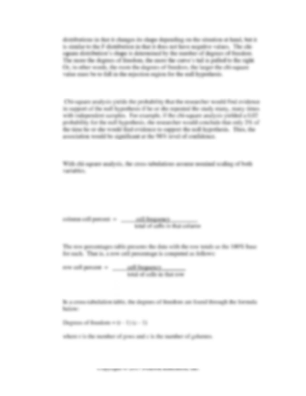
c. Adopting MyPlate eating recommended by the Surgeon General of the United
States for healthful living and family history of heart disease
Diet
Diet
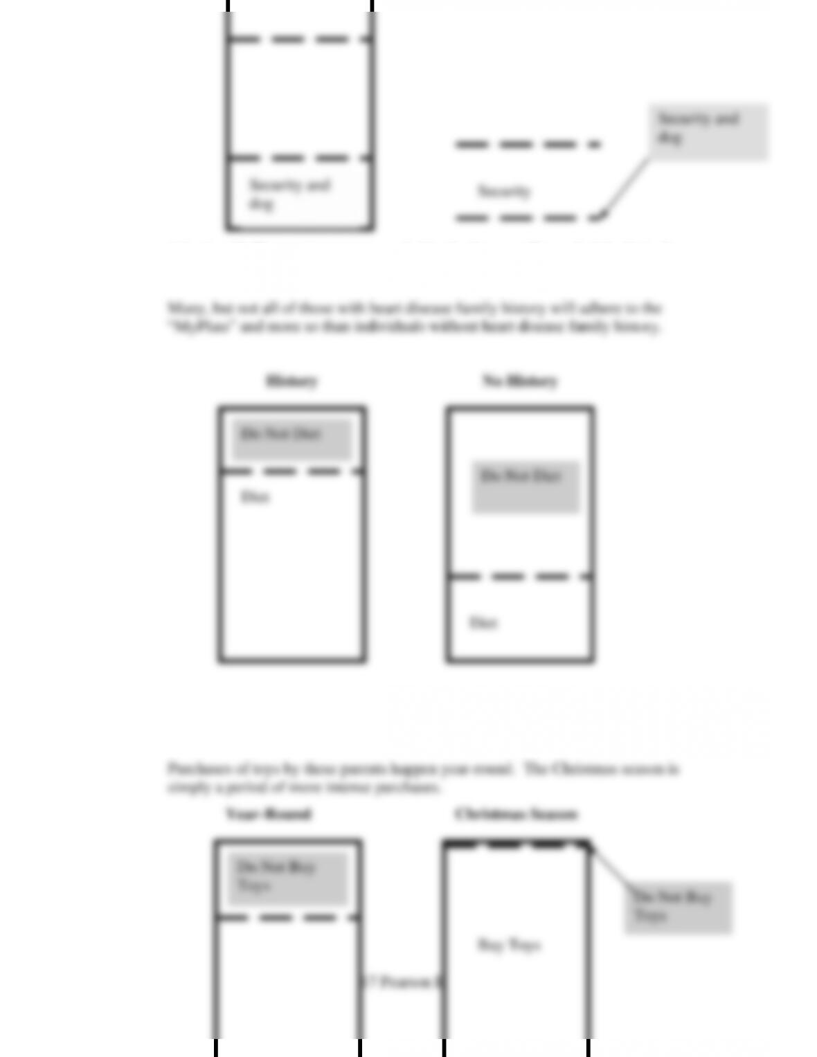
d. Purchases of toys as gifts during the Christmas buying season versus other
seasons of the year by parents of preschool aged children
Security and
dog
Security
Security and
dog
Buy Toys