
CHAPTER 13
IMPLEMENTING BASIC DIFFERENCES TESTS
LEARNING OBJECTIVES
In this chapter you will learn:
13-1 Why difference are important
13-2 How SPSS eliminates the worry of small samples
13-3 To test for significant differences between two groups (percentages and averages)
13-4 Analysis of variance: testing for significant differences in means among more than
two groups
13-5 How to report group differences tests to clients
13-6 To test for differences between two means within the same sample (paired sample
differences)
13-7 The null hypotheses for various differences tests described in this chapter
CHAPTER OUTLINE
Why Differences Are Important
• The differences must be significant
• The differences must be meaningful
• The differences should be stable
• The differences must be actionable
Small Sample Sizes: The Use of a t test or a z test and How SPSS Eliminates the
Worry
Testing for Significant Differences Between Two Groups
• Differences Between Percentages with Two Groups (Independent Samples)
• How to Use SSPS for Differences Between Percentages of Two Groups
• Differences between Means with Two Groups (Independent Samples)
Testing for Significant Differences in Means Among More Than Two
Groups: Analysis of Variance
• Basics of Analysis of Variance
• Post Hoc Tests: Detect Statistically Significant Differences Among Group Means

• Interpreting ANOVA (Analysis of Variance)
Reporting Group Differences Tests to Clients
Differences Between Two Means Within the Same Sample (Paired Sample)
Null Hypotheses for Differences Test Summary
KEY TERMS
Statistical significance of differences Meaningful difference
Stable difference Actionable difference
t test z test
Null hypothesis
Significance of differences between two percentages
Significance of difference between two means
ANOVA (analysis of variance) “Green light” procedure
Post hoc tests Duncan’s multiple range test
One-way ANOVA Group comparison table
Paired samples test for the difference between two means
TEACHING SUGGESTIONS
1. This chapter perpetuates the improvement over previous versions of the textbook
instituted in the fourth edition. Prior editions which included confidence intervals,
hypothesis tests, mean differences, and ANOVA in a single, long chapter. Also, there
are fewer statistical differences formulas although those that remain are simplified
somewhat. Greater emphasis is placed on identifying and interpreting relevant parts
of SPSS output. Hopefully, instructors will find this material less difficult for
students to understand and easier to teach.

2. The chapter begins by claiming that market segmentation is a very important and the
basis for market researchers to investigate statistically significant differences among
identifiable groups of consumers. One may use one’s favorite or most familiar
market segmentation example to augment or emphasize the segmentation differences
central point.
To identify market segments is only the beginning point of the marketing research
notion of significant differences. Once the segments are identified, marketing
research requires that data be gathered about the consumption patterns of the market
segments, and then, these patterns are assessed statistically for significant differences.
The statistical concepts used to compare segments are percentages and means.
It is important to emphasize that marketing segmentation is a conceptual notion, for
whereas segments can be identified in a great many ways, they are not managerially
relevant until statistically significant differences between them are shown that are
useful from a marketing strategy standpoint.
As a simple example, take a florist that segments the local market by geographic area:
North, East, West, and South. The average dollars spent per purchase is calculated
for three flower-giving days in the year. Assume that differences of ±$5 are not
significant.
Area Father’s Day Mother’s Day Valentine’s Day
North $20 $17 $50
East $21 $31 $14
West $15 $17 $25
South $55 $36 $10
What are the promotional implications of these findings?
Answer by day.
Father’s Day – promote heavily to the South
Mother’s Day – promote heavily to the South and East
Valentine’s Day – Promote heavily to the North, moderately to the West and lightly
to the East and South
3. The differences between groups is taken with percentages first because the formulas
are less complicated, and students can relate to them easier than they can relate to the
means differences formulas. The chapter moves quickly from percentage differences
to means differences to SPSS independent samples t test procedure because the intent
is to have students understand the SPSS output and not become bogged down on
computations. Instructors who are more concerned with their students’ learning of

the formulas may wish to dwell longer on the formulas and have students do in-class
or other exercises that require them to use these formulas correctly.
4. Students sometimes appear traumatized by their experiences in their business
statistics course. The section on “Small Sample Sizes: The Use of a t Test or a z Test
and How SPSS Eliminates the Worry” is included to convince students that SPSS will
always issue the proper statistical significance level. It may be valuable to go over
this section at least briefly to help students understand that they are not responsible
for determining the proper statistic and how to look up its significance.
5. The “flag waving” Marketing Research Insight is not meant to be simply “cute.”
Students often find statistical concepts and terminology intimidating, and the flag
waving analogy gives them something tangible to lock onto. The authors, of course,
realize that statistical significance is greatly affected by sample size, and the flag
waving MRI does not admit to the role of sample size. The intent it to give students a
signal as to when to look further into the post hoc findings. This signal is especially
useful for cross-tabulation and correlation treated in chapter 18 (next) because
students typically overlook the significance test with these analyses. If they learn the
signal with differences tests, this learning is generalizable to working with associative
and predictive analyses.
6. The assumption of equal variances in the two samples of a t test for the significance
of the difference between two means is not discussed in the text’s coverage of these
computations. However, students will encounter it when they perform t tests with
SPSS for Windows. The description includes comments on “Levene’s Test for
Equality of Variances,” which is included in the SPSS output for a t test. Instructors
who wish may want to cover the equal variances assumption test in class presentation
and introduce students to the formulas with their own materials.
7. The paired samples t test procedure is much less commonly used than is the
independent samples t test. The latter is the basis for finding statistically significant
differences between two groups (market segments), while the pair samples test
determines differences within a market segment. For example, males may differ from
females on their satisfaction with an online catalog purchasing system, determined via
an independent samples t test. At the same time males may prefer to purchase catalog
items online more than on the telephone, and this would be determined using a
paired-samples t test. Women, although a separate market segment, may prefer
telephone purchases over online purchases with catalog items.
8. The description of one-way analysis of variance is not in depth. Instructors who
desire students to have more knowledge of ANOVA may use this description as a
foundation and move to a more in-depth coverage with their own materials. SPSS for
Windows will accommodate advanced use of one-way and n-way ANOVA.
9. The Duncan’s Multiple Range post hoc test was selected above other post hoc tests
due to its descriptive presentation of significant differences between group means.

The tests not discussed can be assigned to individual students with the requirement to
perform background research and to make a presentation of their findings on the test
to the class. Alternatively, instructors may want to assign students the task of
performing various post hoc tests with SPSS for Windows and comparing their
findings.
ACTIVE LEARNING EXERCISES
Calculations to Determine Significant Differences Between Percents
The calculations are provided in the last column. Note that the frequencies have been
computed to percentages in the table. The only statistically significant difference is in FM
radio ads where the computed z is 2.40 and greater than the 95% level of confidence z of
1.96.
Joined
Did not Join
Difference Finding
Total
100
30
Recall newspaper
ads
45
(45%)
15
(50%)
48.
39.10
5
33.8375.24
5
30
5050
100
5545
5045
21
21
=
+
=
+
−
=
−
=
−
xx
s
pp
z
pp
Recall FM radio
station ads
89
(89%)
20
(67%)
40.2
13.9
22
7.7379.9
22
30
3367
100
1189
6789
21
21
=
+
=
+
−
=
−
=
−
xx
s
pp
z
pp
Recall Yellow
Pages ads
16
(16%)
5
(17%)
13.
77.7
1
03.4744.13
1
30
8317
100
8416
1716
21
21
=
+
=
+
−
=
−
=
−
xx
s
pp
z
pp
Recall local TV
news ads
21
(21%)
6
(20%)
12.
36.8
1
55.5359.16
1
30
8020
100
7921
2021
21
21
=
+
=
+
−
=
−
=
−
xx
s
pp
z
pp
Perform Means Differences Analysis with SPSS
For this Active Learning exercise, determine if there is a difference in the preferences for
the various possible hybrid models based on gender. That is, redo the one-seat, three-
wheel hybrid model just to make sure that you can find and execute the analysis. Then
use the clickstream instructions in Figure 17.2 to direct SPSS to perform this analysis for
each of the other possible hybrid models, and use the annotations on the Independent
Samples T-Test output provided in Figure 17.3 to interpret your findings.
Group Statistics
Gender
N
Mean
Std. Deviation
Std. Error Mean
Preference: Super Cycle 1
seat hybrid
Male
505
3.50
1.697
.076
Female
495
3.09
1.768
.079
Preference: Runabout Sport
2 seat hybrid
Male
505
4.24
1.710
.076
Female
495
4.29
1.714
.077
Preference: Runabout with
Male
505
3.85
1.856
.083
Luggage 2 seat hybrid
Female
495
3.72
1.877
.084
Preference: Economy 4 seat
hybrid
Male
505
3.54
1.851
.082
Female
495
3.45
1.827
.082
Preference: Standard 4 seat
hybrid
Male
505
4.82
1.582
.070
Female
495
5.10
1.659
.075
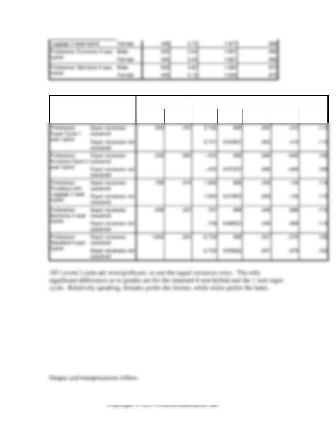
Independent Samples Test
Levene’s Test for
Equality of Variances
t-test for Equality of Means
F
Sig.
t
df
Sig. (2-
tailed)
Mean
Difference
Std. Error
Difference
Preference:
Super Cycle 1
seat hybrid
Equal variances
assumed
.093
.761
3.742
998
.000
.410
.110
Equal variances not
assumed
3.741
9.943E2
.000
.410
.110
Preference:
Runabout Sport 2
seat hybrid
Equal variances
assumed
.000
.985
-.455
998
.649
-.049
.108
Equal variances not
assumed
-.455
9.975E2
.649
-.049
.108
Preference:
Runabout with
Luggage 2 seat
hybrid
Equal variances
assumed
.790
.374
1.053
998
.293
.124
.118
Equal variances not
assumed
1.053
9.970E2
.293
.124
.118
Preference:
Economy 4 seat
hybrid
Equal variances
assumed
.649
.421
.757
998
.449
.088
.116
Equal variances not
assumed
.758
9.980E2
.449
.088
.116
Preference:
Standard 4 seat
hybrid
Equal variances
assumed
1.634
.201
-2.724
998
.007
-.279
.102
Equal variances not
assumed
-2.723
9.935E2
.007
-.279
.103
All Levene’s tests are nonsiginficant, so use the equal variances rows. The only
significant differences as to gender are for the standard 4 seat hybrid and the 1 seat super
cycle. Relatively speaking, females prefer the former, while males prefer the latter.
Perform Analysis of Variance with SPSS
Let’s investigate for age-group means differences across all of the hybrid models under
consideration at this time by Advanced Automobile Concepts. We recommend that you
use the AAConcepts.sav data set and run the ANOVA just described. Make sure that your
SPSS output looks like that in Figure 17.5. Then investigate the preference mean
differences for the other hybrid models by age group.
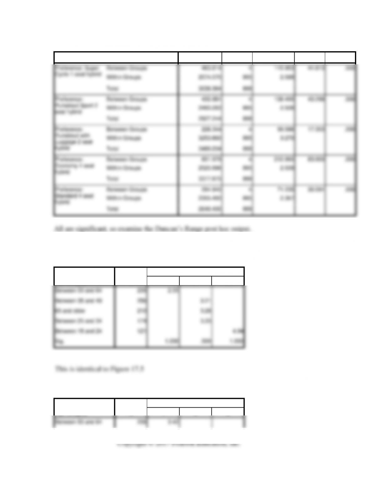
ANOVA
Sum of Squares
df
Mean Square
F
Sig.
Preference: Super
Cycle 1 seat hybrid
Between Groups
463.814
4
115.953
44.813
.000
Within Groups
2574.570
995
2.588
Total
3038.384
999
Preference:
Runabout Sport 2
seat hybrid
Between Groups
433.981
4
108.495
43.298
.000
Within Groups
2493.263
995
2.506
Total
2927.244
999
Preference:
Runabout with
Luggage 2 seat
hybrid
Between Groups
226.344
4
56.586
17.303
.000
Within Groups
3253.860
995
3.270
Total
3480.204
999
Preference:
Economy 4 seat
hybrid
Between Groups
851.979
4
212.995
83.900
.000
Within Groups
2525.996
995
2.539
Total
3377.975
999
Preference:
Standard 4 seat
hybrid
Between Groups
284.940
4
71.235
30.091
.000
Within Groups
2355.460
995
2.367
Total
2640.400
999
All are significant, so examine the Duncan’s Range post hoc output.
Post Hoc Tests
Preference: Super Cycle 1 seat hybrid
Duncana,,b
Age category
N
Subset for alpha = 0.05
1
2
3
Between 50 and 64
239
2.55
Between 35 and 49
256
3.21
65 and older
210
3.28
Between 25 and 34
174
3.33
Between 18 and 24
121
4.94
Sig.
1.000
.500
1.000
This is identical to Figure 17.5
Preference: Runabout Sport 2 seat hybrid
Duncana,,b
Age category
N
Subset for alpha = 0.05
1
2
3
Between 50 and 64
239
3.42
Between 25 and 34
174
4.17
Between 35 and 49
256
4.34
65 and older
210
4.37
Between 18 and 24
121
5.73
Sig.
1.000
.242
1.000
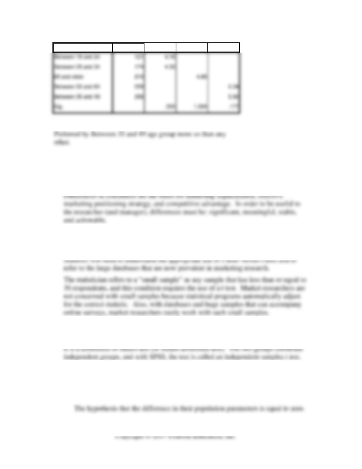
Preferred by Between 18 and 24 age group more so than any
other.
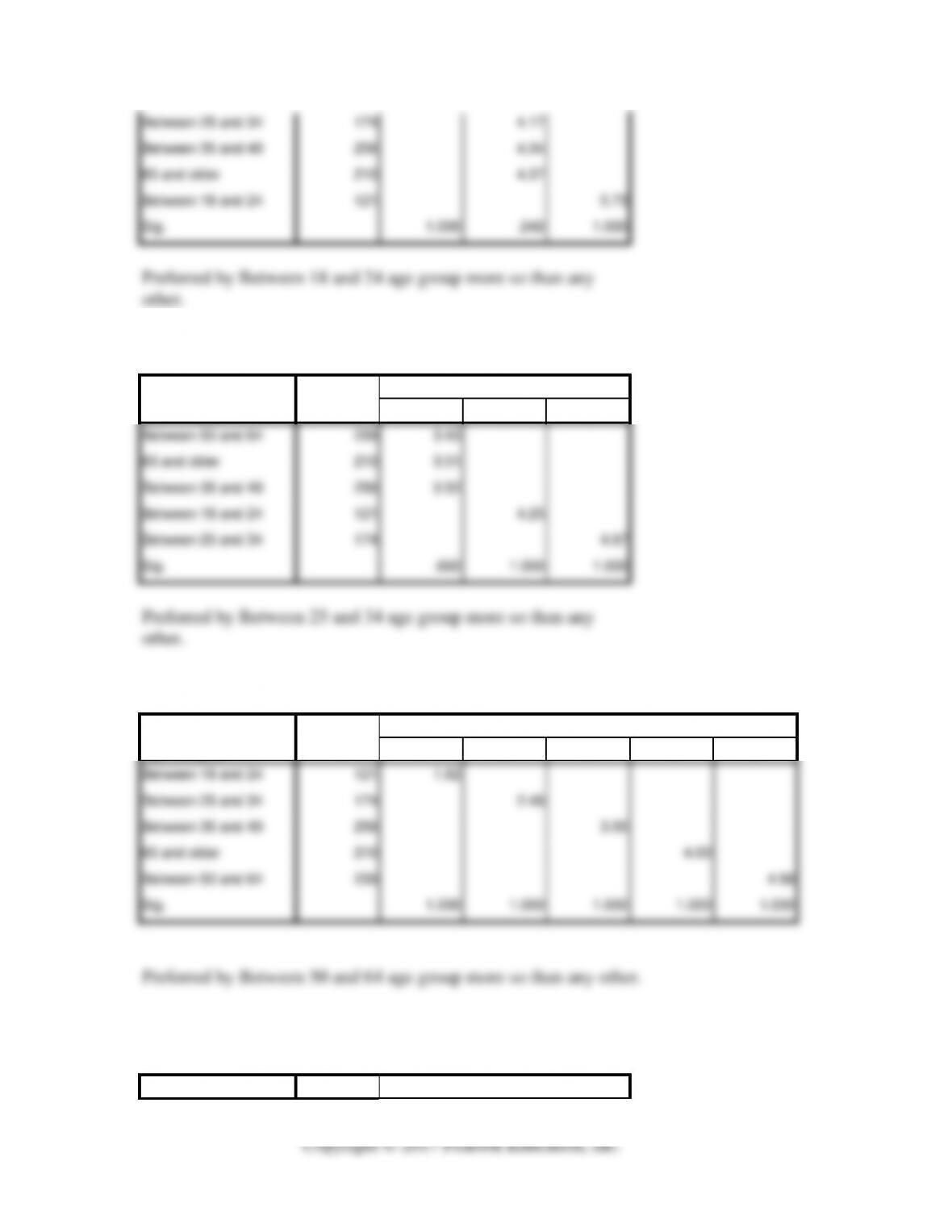
Preference: Runabout with Luggage 2 seat hybrid
Duncana,,b
Age category
N
Subset for alpha = 0.05
1
2
3
Between 50 and 64
239
3.43
65 and older
210
3.51
Between 35 and 49
256
3.52
Between 18 and 24
121
4.25
Between 25 and 34
174
4.67
Sig.
.660
1.000
1.000
Preferred by Between 25 and 34 age group more so than any
other.
Preference: Economy 4 seat hybrid
Duncana,,b
Age category
N
Subset for alpha = 0.05
1
2
3
4
5
Between 18 and 24
121
1.82
Between 25 and 34
174
2.48
Between 35 and 49
256
3.55
65 and older
210
4.00
Between 50 and 64
239
4.58
Sig.
1.000
1.000
1.000
1.000
1.000
Preferred by Between 50 and 64 age group more so than any other.
Preference: Standard 4 seat hybrid
Duncana,,b
Age category
N
Subset for alpha = 0.05
1
2
3
Between 18 and 24
121
4.16
Between 25 and 34
174
4.30
65 and older
210
4.80
Between 50 and 64
239
5.34
Between 35 and 49
256
5.56
Sig.
.355
1.000
.177
Preferred by Between 35 and 49 age group more so than any
other.
ANSWERS TO REVIEW QUESTIONS/APPLICATIONS
1. What are differences and why should market researchers be concerned with them?
Why are marketing managers concerned with them?
2. What is considered to be a “small sample,” and why is this concept a concern to
statisticians? To what extent do market researchers concern themselves with small
samples? Why?
3. When a market researcher compares the responses of two identifiable groups with
respect to their answers to the same question, what is this called?
4. With regard to differences tests, briefly define and describe each of the following:
a. Null hypothesis

b. Sampling distribution
c. Significant difference
5. Relate the formula and identify each formula’s components in the test of significant
differences between two groups when the question involved is…
a. a “yes/no” type.
21
21
pp
s
pp
z
−
−
=
Where:
1
p
= percentage found in sample 1
2
p
= percentage found in sample 2
21 pp
s−
= standard error of the difference between two percentages
b. a scale variable question.

21
21
xx
s
xx
z
−
−
=
Where:
=
1
x
mean found in sample 1
=
2
x
mean found in sample 2
21 xx
s−
= standard error of the difference between two means
6. For each of the following three cases (a-c) are the two sample results significantly
different?
Sample Sample Confidence Your
One Two Level Finding?_____
Mean: 10.6 Mean: 11.7 95%
Std. dev:1.5 Std. dev: 2.5
n = 150 n = 300
The computed z is greater than 1.96, so the difference is significant at the 95% level.
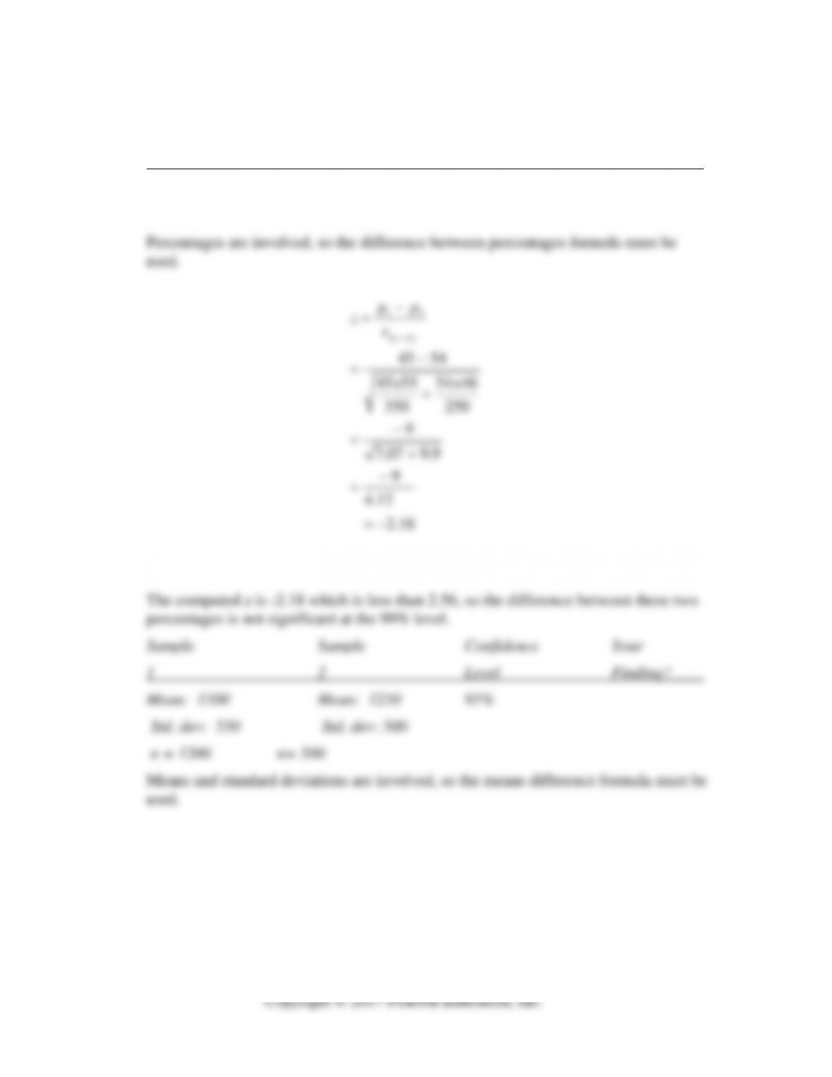
Sample Sample Confidence Your
1 2 Level Finding?____
Percent: 45% Percent: 54% 99%
n = 350 n = 250
18.2
12.4
9
9.907.7
9
250
4654
350
5545
5445
21
21
−=
−
=
+
−
=
+
−
=
−
=
−
xx
s
pp
z
pp
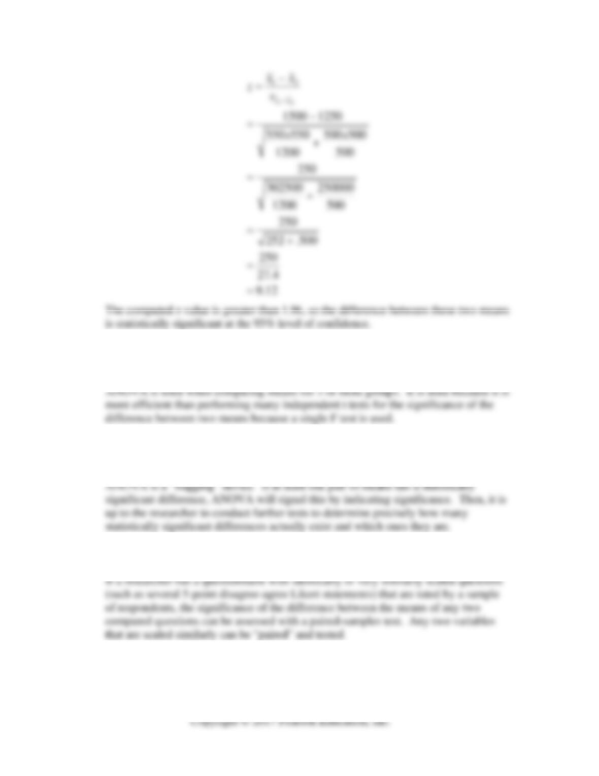
12.9
4.27
250
500.252
250
500
250000
1200
302500
250
500
500500
1200
550550
12501500
21
21
=
=
+
=
+
=
+
−
=
−
=
−
xx
s
xx
z
xx
The computed z value is greater than 1.96, so the difference between these two means
is statistically significant at the 95% level of confidence.
7. When should one-way ANOVA be used and why?
8. When a researcher finds a significant F value in an analysis of variance, why may it
be considered a “green light” device?
9. What is a paired-samples test? Specifically how are the samples “paired”?
10. The Circulation Manager of the Daily Advocate newspaper commissions a market
research study to determine what factors underlie the circulation attrition.
Specifically, the survey is designed to compare current Daily Advocate subscribers

with those who have dropped their subscriptions in the past year. A telephone survey
is conducted with both sets of individuals. Following is a summary of the key findings
from the study. Interpret these findings for the circulation manager.
Item
Current
Subscribers
Lost
Subscribers
Significance
B Length of residence in the city
20.1 yrs
5.4 yrs
.000
Length of time as a subscriber
27.2 yrs
1.3 yrs
.000
Watch local TV news program (s)
87%
85%
.372
Watch national news program(s)
72%
79%
.540
Obtain news from the Internet
13%
23%
.025
Satisfaction* with…
Delivery of newspaper
5.5
4.9
.459
Coverage of local news
6.1
5.8
.248
Coverage of national news
5.5
2.3
.031
Coverage of local sports
6.3
5.9
.462
Coverage of national sports
5.7
3.2
.001
Coverage of local social news
5.8
5.2
.659
Editorial stance of the newspaper
6.1
4.0
.001
Value for subscription price
5.2
4.8
.468
*Based on a 7-point scale where 1=very dissatisfied and 7=very satisfied
Interpret these findings for the Circulation Manager.
11. A researcher is investigating different types of customers for a sporting goods store.
In a survey, respondents are asked to use their Fitbit devices to indicate how much
they exercised last week using categories of “Less than 1 hour,” “Between 1 and 2
hours,” “Between 2 and 3 hours,” and so on. These respondents have also rated the
performance of the sporting goods store across 12 characteristics, such as good
value for the price, convenience of location, helpfulness of the sales clerks, and so on.
The researcher used a 7-point rating scale for these 12 characteristics where 1 =
Poor performance to 7 = Excellent performance. How can the researcher investigate
differences in the ratings based on the amount of exercise reported by the
respondents?

12. A marketing manager of newegg, a web-based electronic products sales company,
uses a segmentation scheme based on the incomes of target customers. The
segmentation system has four segments: (1) low income, (2) moderate income, (3)
high income, and (4) wealthy. The company database holds information on
customers’ purchases over the past several months. Using Microsoft Excel on this
database, the marketing manager finds that the average total dollar purchases for the
four groups are as follows.
Market Segment Average Total Dollar Purchases
Low income $101
Moderate income $120
High income $231
Wealthy $595
Construct a table that is based on the Duncan’s multiple range test table concept
discussed in the chapter that illustrates that the low and moderate income groups are
not different from each other, but the other groups are significantly different from one
another.
CASE SOLUTIONS
Case 13.1 L’Experience Félicité Restaurant Survey Differences Analysis
Case Objective
The objective of the L’Experience Félicité Restaurant survey case is to have students
identify what differences tests are appropriate, to run them, and interpret them correctly.
Answers to Case Questions
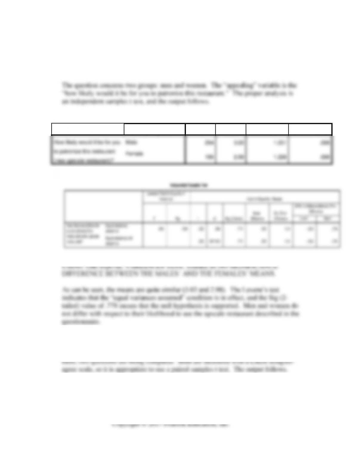
1. Jeff wonders if L’Experience Félicité Restaurant is more appealing to women that it
is to men or vice versa. Perform the proper analysis, interpret it, and answer Jeff’s
question.
Group Statistics
What is your gender?
N
Mean
Std. Deviation
Std. Error Mean
How likely would it be for you
to patronize this restaurant
(new upscale restaurant)?
Male
204
3.02
1.251
.088
Female
196
2.98
1.226
.088
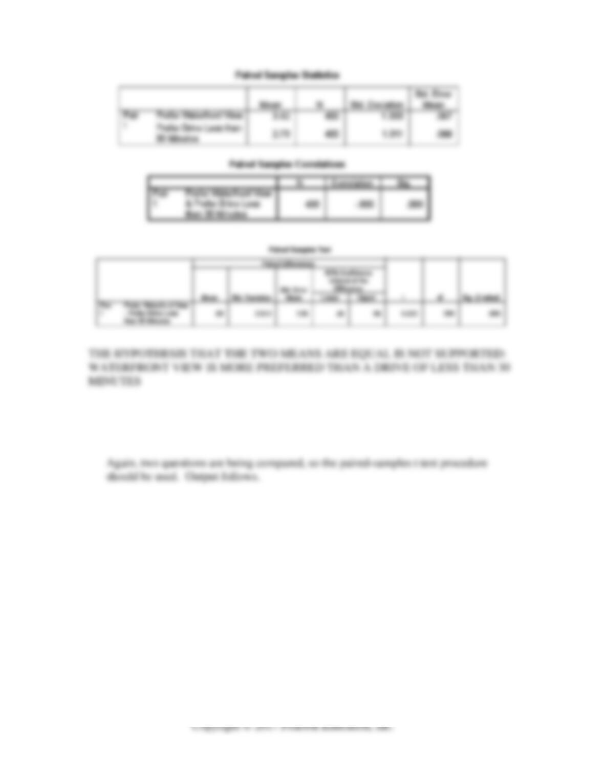
2. With respect to the location of L’Experience Félicité Restaurant, is a waterfront view
preferred more than a drive of less than 30 minutes?
3. With respect to the restaurant’s atmosphere is a string quartet preferred over a jazz
combo?