Frequency
Percent
Valid Percent
Cumulative
Percent
Valid
Less than High School
11
2.8
2.8
2.8
Some High School
14
3.5
3.5
6.3
High School Graduate
14
3.5
3.5
9.8
Some College (No Degree)
14
3.5
3.5
13.3
Associate Degree
14
3.5
3.5
16.8
Bachelor’s Degree
238
59.5
59.5
76.3
Master’s Degree
86
21.5
21.5
97.8
Doctorate Degree
9
2.3
2.3
100.0
Total
400
100.0
100.0
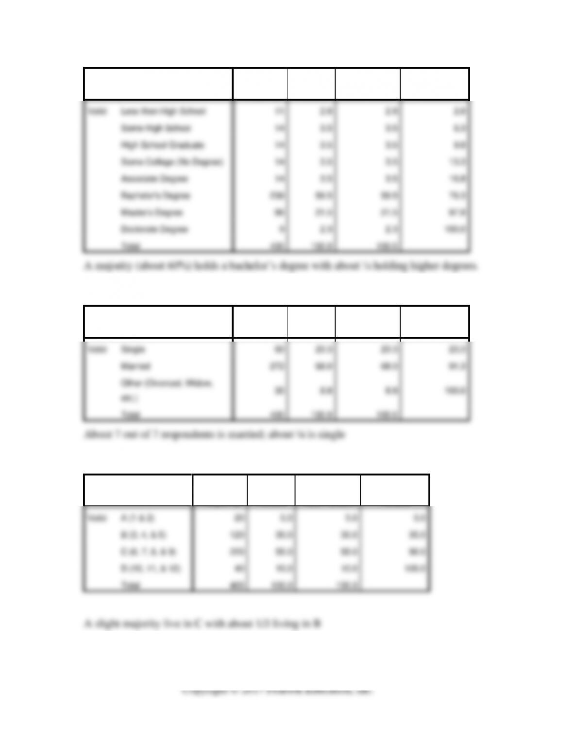
A majority (about 60%) holds a bachelor’s degree with about ¼ holding higher degrees.
What is your marital status?
Frequency
Percent
Valid Percent
Cumulative
Percent
Valid
Single
93
23.3
23.3
23.3
Married
272
68.0
68.0
91.3
Other (Divorced, Widow,
etc.)
35
8.8
8.8
100.0
Total
400
100.0
100.0
About 7 out of 7 respondents is married; about ¼ is single
Please check the letter that includes the Zip Code in which you live (coded by letter).
Frequency
Percent
Valid Percent
Cumulative
Percent
Valid
A (1 & 2)
20
5.0
5.0
5.0
B (3, 4, & 5)
120
30.0
30.0
35.0
C (6, 7, 8, & 9)
220
55.0
55.0
90.0
D (10, 11, & 12)
40
10.0
10.0
100.0
Total
400
100.0
100.0
A slight majority live in C with about 1/3 living in B
Which of the following categories best describes your before tax household income?
Frequency
Percent
Valid Percent
Cumulative
Percent
Valid
<$15,000
26
6.5
6.5
6.5
$15,000 to $24,999
34
8.5
8.5
15.0
$25,000 to $49,999
82
20.5
20.5
35.5
$50,000 to $74,999
133
33.3
33.3
68.8
$75,000 to $99,999
16
4.0
4.0
72.8
$100,000 to $149,999
43
10.8
10.8
83.5
$150,000+
66
16.5
16.5
100.0
Total
400
100.0
100.0
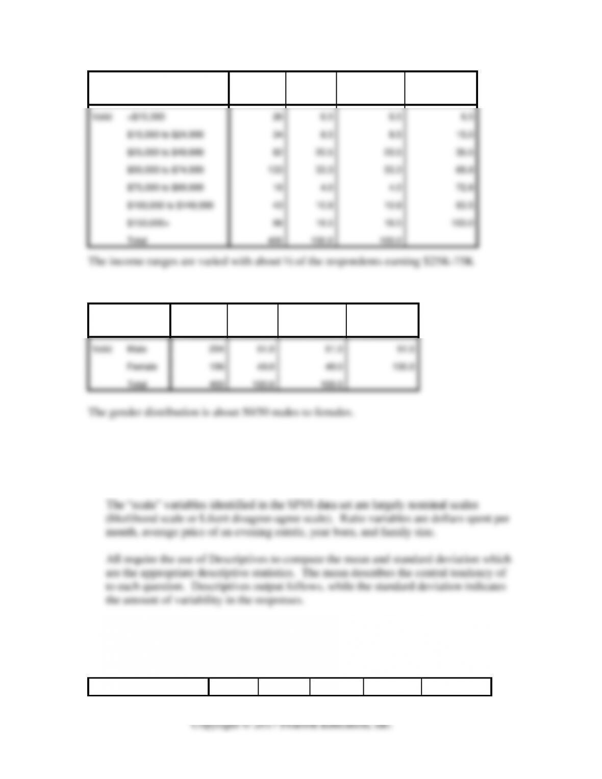
The income ranges are varied with about ½ of the respondents earning $25K-75K
What is your gender?
Frequency
Percent
Valid Percent
Cumulative
Percent
Valid
Male
204
51.0
51.0
51.0
Female
196
49.0
49.0
100.0
Total
400
100.0
100.0
The gender distribution is about 50/50 males to females.
2. Determine what variables are scale variables (either interval or ratio scales),
perform the appropriate descriptive analysis, and interpret it.
Descriptives
Descriptive Statistics
N
Minimum
Maximum
Mean
Std. Deviation
How many total dollars do
you spend per month in
restaurants (for your meals
only)?
400
$5.00
$450.00
$150.0525
$92.70629
What would you expect an
average evening meal
entree item alone to be
priced?
340
$16.00
$70.00
$28.8353
$9.82784
Valid N (listwise)
340
Descriptive Statistics
N
Minimum
Maximum
Mean
Std. Deviation
How likely would it be for
you to patronize this
restaurant (new upscale
restaurant)?
400
1
5
3.00
1.237
Valid N (listwise)
400
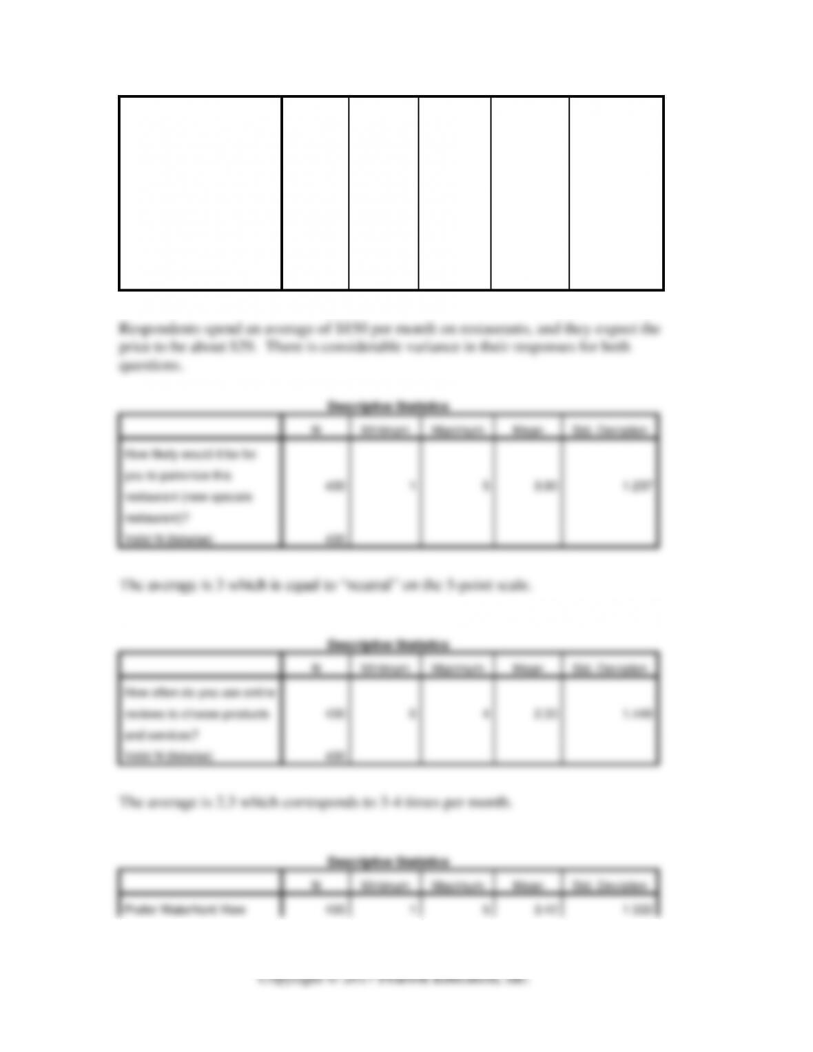
The average is 3 which is equal to “neutral” on the 5-point scale.
Descriptive Statistics
N
Minimum
Maximum
Mean
Std. Deviation
How often do you use online
reviews to choose products
and services?
400
0
4
2.33
1.449
Valid N (listwise)
400
The average is 2.3 which corresponds to 3-4 times per month.
Descriptive Statistics
N
Minimum
Maximum
Mean
Std. Deviation
Prefer Waterfront View
400
1
5
3.42
1.333
Prefer Drive Less than 30
Minutes
400
1
5
2.73
1.311
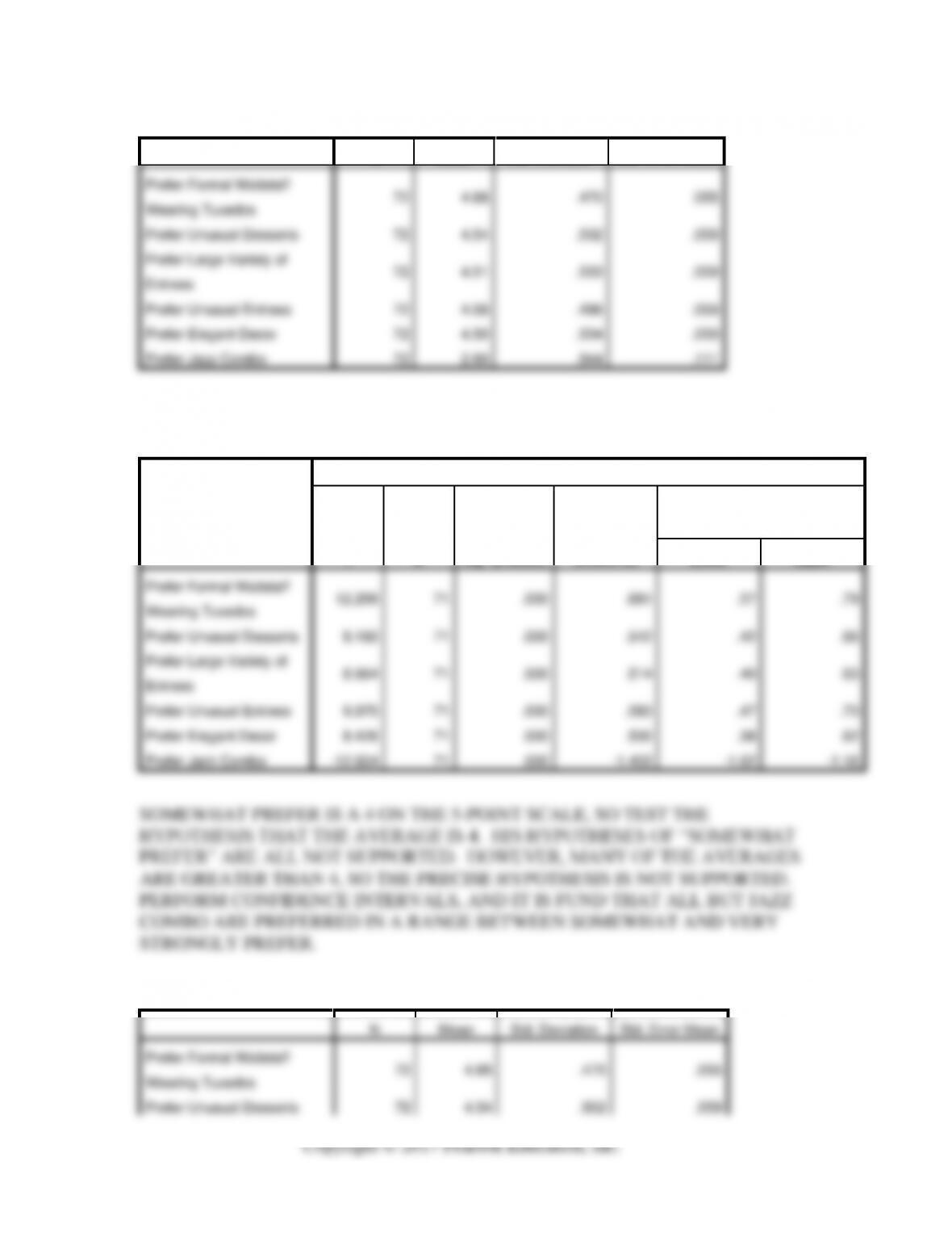
Prefer Formal Waitstaff
Wearing Tuxedos
400
1
5
2.47
1.516
Prefer Unusual Desserts
400
1
5
2.41
1.514
Prefer Large Variety of
Entrees
400
1
5
2.48
1.466
Prefer Unusual Entrees
400
1
5
2.40
1.550
Prefer Simple Decor
400
1
5
3.58
1.492
Prefer Elegant Decor
400
1
5
2.33
1.510
Prefer String Quartet
400
1
5
2.50
1.420
Prefer Jazz Combo
400
1
5
3.69
1.221
Valid N (listwise)
400
Descriptive Statistics
N
Minimum
Maximum
Mean
Std. Deviation
Year Born
400
1943
1990
1972.46
9.516
Valid N (listwise)
400
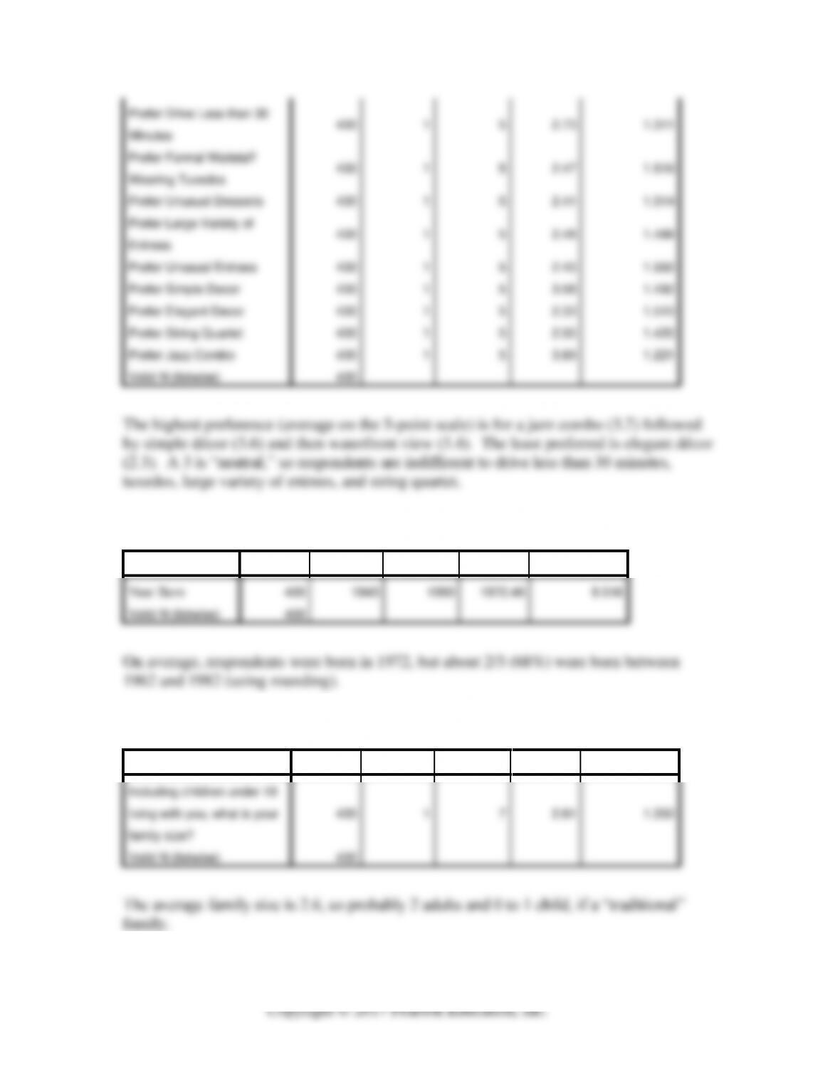
On average, respondents were born in 1972, but about 2/3 (68%) were born between
1962 and 1982 (using rounding).
Descriptive Statistics
N
Minimum
Maximum
Mean
Std. Deviation
Including children under 18
living with you, what is your
family size?
400
1
7
2.61
1.350
Valid N (listwise)
400
The average family size is 2.6, so probably 2 adults and 0 to 1 child, if a “traditional”
family.
3. What are the population estimates for each of the following?
a. Presence for “easy listening” radio programming
b. Viewing of 10:00 p.m. local news on TV
c. Subscribe to City Magazine
d. Average age of heads of households
e. Average price paid for an evening meal entrée
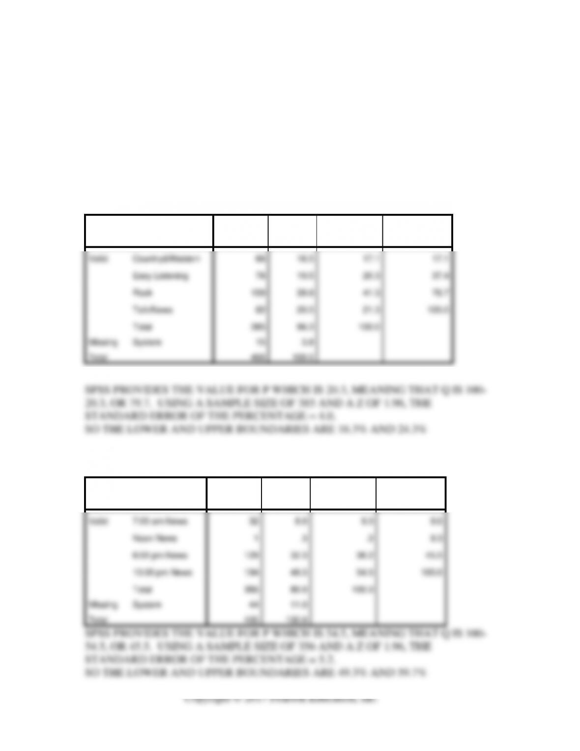
To which type of radio programming do you most often listen?
Frequency
Percent
Valid Percent
Cumulative
Percent
Valid
Country&Western
66
16.5
17.1
17.1
Easy Listening
78
19.5
20.3
37.4
Rock
159
39.8
41.3
78.7
Talk/News
82
20.5
21.3
100.0
Total
385
96.3
100.0
Missing
System
15
3.8
Total
400
100.0
SPSS PROVIDES THE VALUE FOR P WHICH IS 20.3, MEANING THAT Q IS 100–
20.3, OR 79.7. USING A SAMPLE SIZE OF 385 AND A Z OF 1.96, THE
STANDARD ERROR OF THE PERCENTAGE = 4.0.
SO THE LOWER AND UPPER BOUNDARIES ARE 16.3% AND 24.3%
Which newscast do you watch most frequently?
Frequency
Percent
Valid Percent
Cumulative
Percent
Valid
7:00 am News
32
8.0
9.0
9.0
Noon News
1
.3
.3
9.3
6:00 pm News
129
32.3
36.2
45.5
10:00 pm News
194
48.5
54.5
100.0
Total
356
89.0
100.0
Missing
System
44
11.0
Total
400
100.0
SPSS PROVIDES THE VALUE FOR P WHICH IS 54.5, MEANING THAT Q IS 100–
54.5, OR 45.5. USING A SAMPLE SIZE OF 356 AND A Z OF 1.96, THE
STANDARD ERROR OF THE PERCENTAGE = 5.2.
SO THE LOWER AND UPPER BOUNDARIES ARE 49.3% AND 59.7%
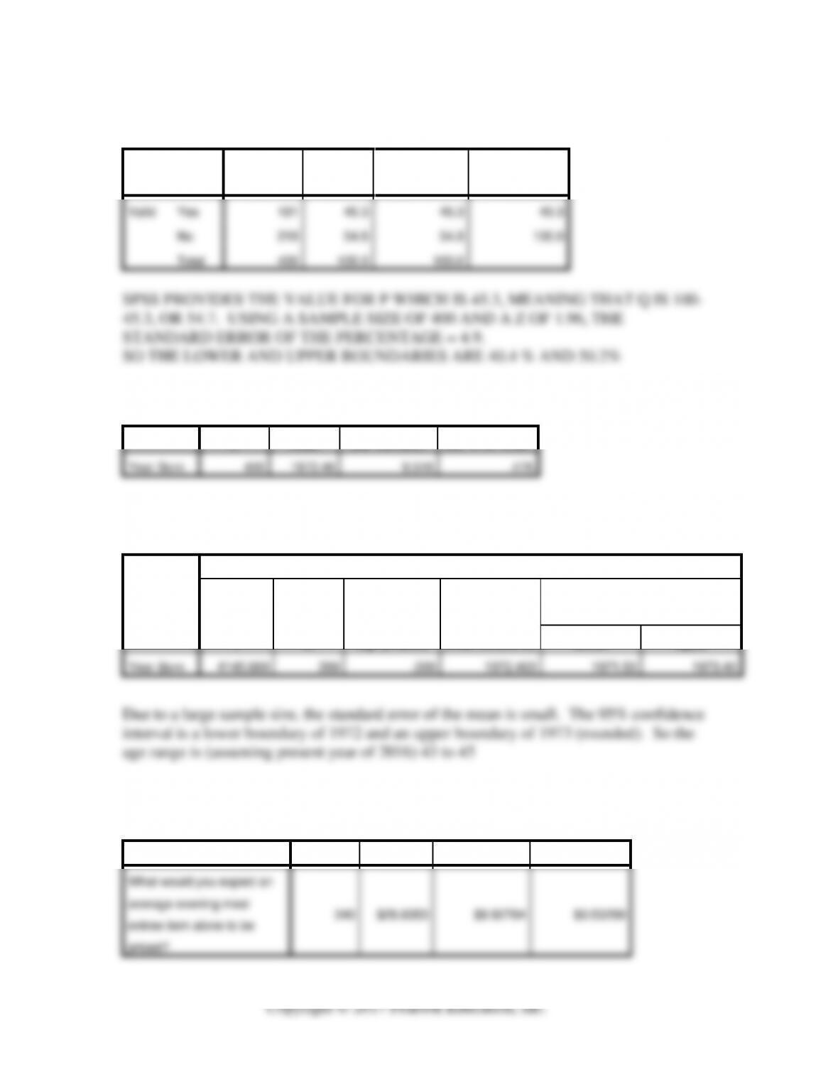
Do you subscribe to City Magazine?
Frequency
Percent
Valid Percent
Cumulative
Percent
Valid
Yes
181
45.3
45.3
45.3
No
219
54.8
54.8
100.0
Total
400
100.0
100.0
SPSS PROVIDES THE VALUE FOR P WHICH IS 45.3, MEANING THAT Q IS 100-
45.3, OR 54.7. USING A SAMPLE SIZE OF 400 AND A Z OF 1.96, THE
STANDARD ERROR OF THE PERCENTAGE = 4.9.
SO THE LOWER AND UPPER BOUNDARIES ARE 40.4 % AND 50.2%
One-Sample Statistics
N
Mean
Std. Deviation
Std. Error Mean
Year Born
400
1972.46
9.516
.476
One-Sample Test
Test Value = 0
t
df
Sig. (2-tailed)
Mean Difference
95% Confidence Interval of the
Difference
Lower
Upper
Year Born
4145.669
399
.000
1972.463
1971.53
1973.40
Due to a large sample size, the standard error of the mean is small. The 95% confidence
interval is a lower boundary of 1972 and an upper boundary of 1973 (rounded). So the
age range is (assuming present year of 2016) 43 to 45
One-Sample Statistics
N
Mean
Std. Deviation
Std. Error Mean
What would you expect an
average evening meal
entree item alone to be
priced?
340
$28.8353
$9.82784
$0.53299
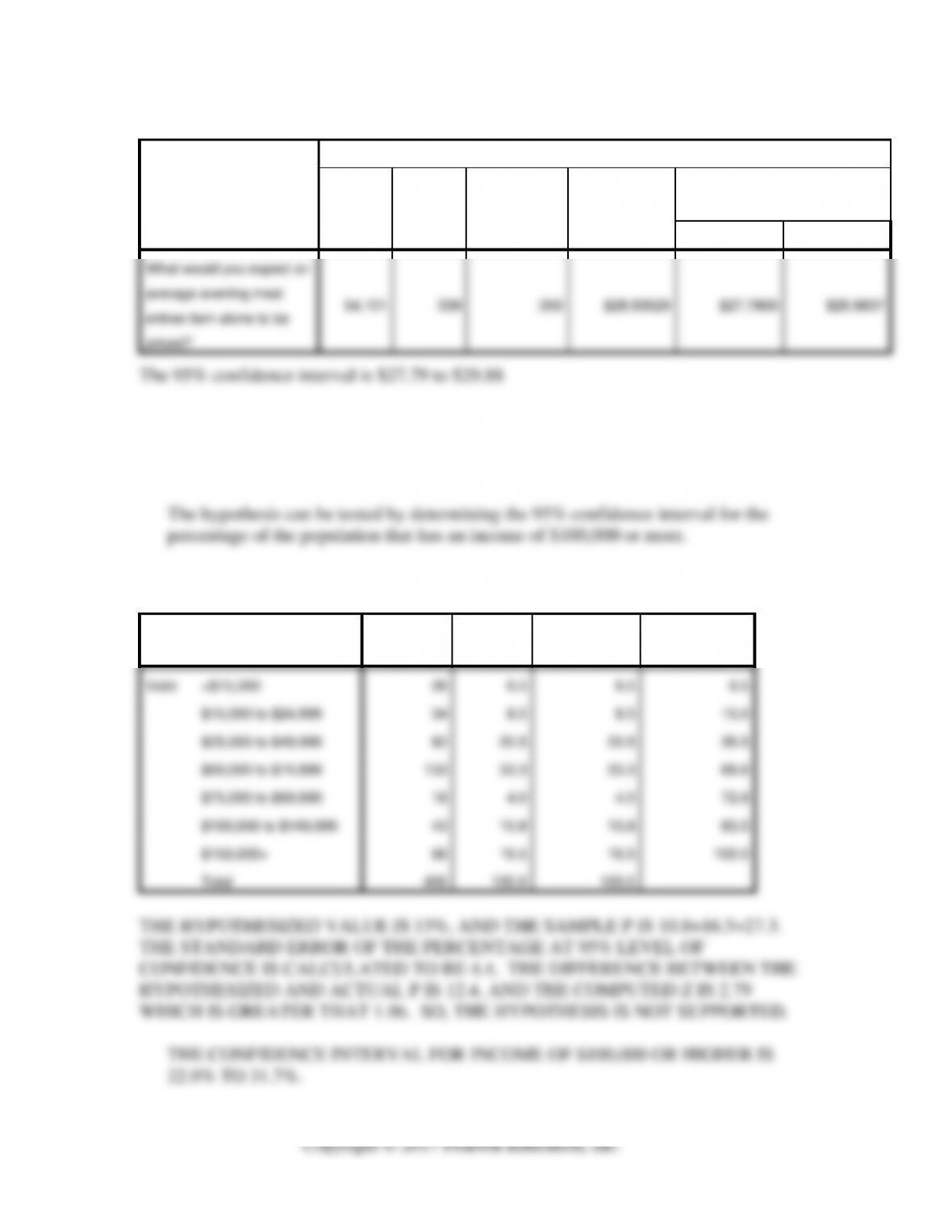
One-Sample Test
Test Value = 0
t
df
Sig. (2-tailed)
Mean
Difference
95% Confidence Interval of the
Difference
Lower
Upper
What would you expect an
average evening meal
entree item alone to be
priced?
54.101
339
.000
$28.83529
$27.7869
$29.8837
The 95% confidence interval is $27.79 to $29.88
4. Because this restaurant will be upscale, it will appeal to high-income consumers.
The investors’ hopes that at least 15% of the households represented in the survey
have an income level of $100,000 or higher. Test this hypothesis.
Which of the following categories best describes your before tax household income?
Frequency
Percent
Valid Percent
Cumulative
Percent
Valid
<$15,000
26
6.5
6.5
6.5
$15,000 to $24,999
34
8.5
8.5
15.0
$25,000 to $49,999
82
20.5
20.5
35.5
$50,000 to $74,999
133
33.3
33.3
68.8
$75,000 to $99,999
16
4.0
4.0
72.8
$100,000 to $149,999
43
10.8
10.8
83.5
$150,000+
66
16.5
16.5
100.0
Total
400
100.0
100.0
THE HYPOTHESIZED VALUE IS 15%, AND THE SAMPLE P IS 10.8+16.5=27.3.
THE STANDARD ERROR OF THE PERCENTAGE AT 95% LEVEL OF
CONFIDENCE IS CALCULATED TO BE 4.4. THE DIFFERENCE BETWEEN THE
HYPOTHESIZED AND ACTUAL P IS 12.4, AND THE COMPUTED Z IS 2.79
WHICH IS GREATER THAT 1.96. SO, THE HYPOTHESIS IS NOT SUPPORTED.
5. With respect to those who are “very likely” to patronize the L’Experience Félicite
Restaurant, Jeff believes that they will either “very strongly” or “somewhat” prefer
each of the following: (a) waitstaff with tuxedos, (b) unusual desserts, (c) large
variety of entrees, (d) unusual entrees, (e) elegant décor, and (f) jazz combo music.
Does the survey support or refute Jeff’s hypotheses? Interpret your findings.
This analysis first requires that only respondents who are “very likely” to patronize
the L’Experience Félicité Restaurant be selected from the larger sample.
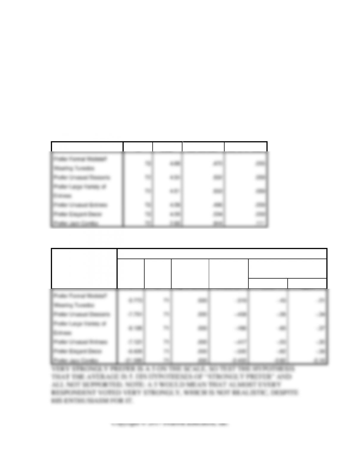
One-Sample Statistics
N
Mean
Std. Deviation
Std. Error Mean
Prefer Formal Waitstaff
Wearing Tuxedos
72
4.68
.470
.055
Prefer Unusual Desserts
72
4.54
.502
.059
Prefer Large Variety of
Entrees
72
4.51
.503
.059
Prefer Unusual Entrees
72
4.58
.496
.059
Prefer Elegant Decor
72
4.50
.504
.059
Prefer Jazz Combo
72
2.60
.944
.111
One-Sample Test
Test Value = 5
t
df
Sig. (2-tailed)
Mean
Difference
95% Confidence Interval of the
Difference
Lower
Upper
Prefer Formal Waitstaff
Wearing Tuxedos
-5.773
71
.000
-.319
-.43
-.21
Prefer Unusual Desserts
-7.751
71
.000
-.458
-.58
-.34
Prefer Large Variety of
Entrees
-8.195
71
.000
-.486
-.60
-.37
Prefer Unusual Entrees
-7.121
71
.000
-.417
-.53
-.30
Prefer Elegant Decor
-8.426
71
.000
-.500
-.62
-.38
Prefer Jazz Combo
-21.589
71
.000
-2.403
-2.62
-2.18
VERY STRONGLY PREFER IS A 5 ON THE SCALE, SO TEST THE HYPOTHESIS
THAT THE AVERAGE IS 5. HIS HYPOTHESES OF “STRONGLY PREFER” AND
ALL NOT SUPPORTED. NOTE: A 5 WOULD MEAN THAT ALMOST EVERY
RESPONDENT VOTED VERY STRONGLY, WHICH IS NOT REALISTIC, DESPITE
HIS ENTHUSIASM FOR IT.
One-Sample Statistics
N
Mean
Std. Deviation
Std. Error Mean
Prefer Formal Waitstaff
Wearing Tuxedos
72
4.68
.470
.055
Prefer Unusual Desserts
72
4.54
.502
.059
Prefer Large Variety of
Entrees
72
4.51
.503
.059
Prefer Unusual Entrees
72
4.58
.496
.059
Prefer Elegant Decor
72
4.50
.504
.059
Prefer Jazz Combo
72
2.60
.944
.111
One-Sample Test
Test Value = 4
t
df
Sig. (2-tailed)
Mean
Difference
95% Confidence Interval of the
Difference
Lower
Upper
Prefer Formal Waitstaff
Wearing Tuxedos
12.299
71
.000
.681
.57
.79
Prefer Unusual Desserts
9.160
71
.000
.542
.42
.66
Prefer Large Variety of
Entrees
8.664
71
.000
.514
.40
.63
Prefer Unusual Entrees
9.970
71
.000
.583
.47
.70
Prefer Elegant Decor
8.426
71
.000
.500
.38
.62
Prefer Jazz Combo
-12.604
71
.000
-1.403
-1.62
-1.18
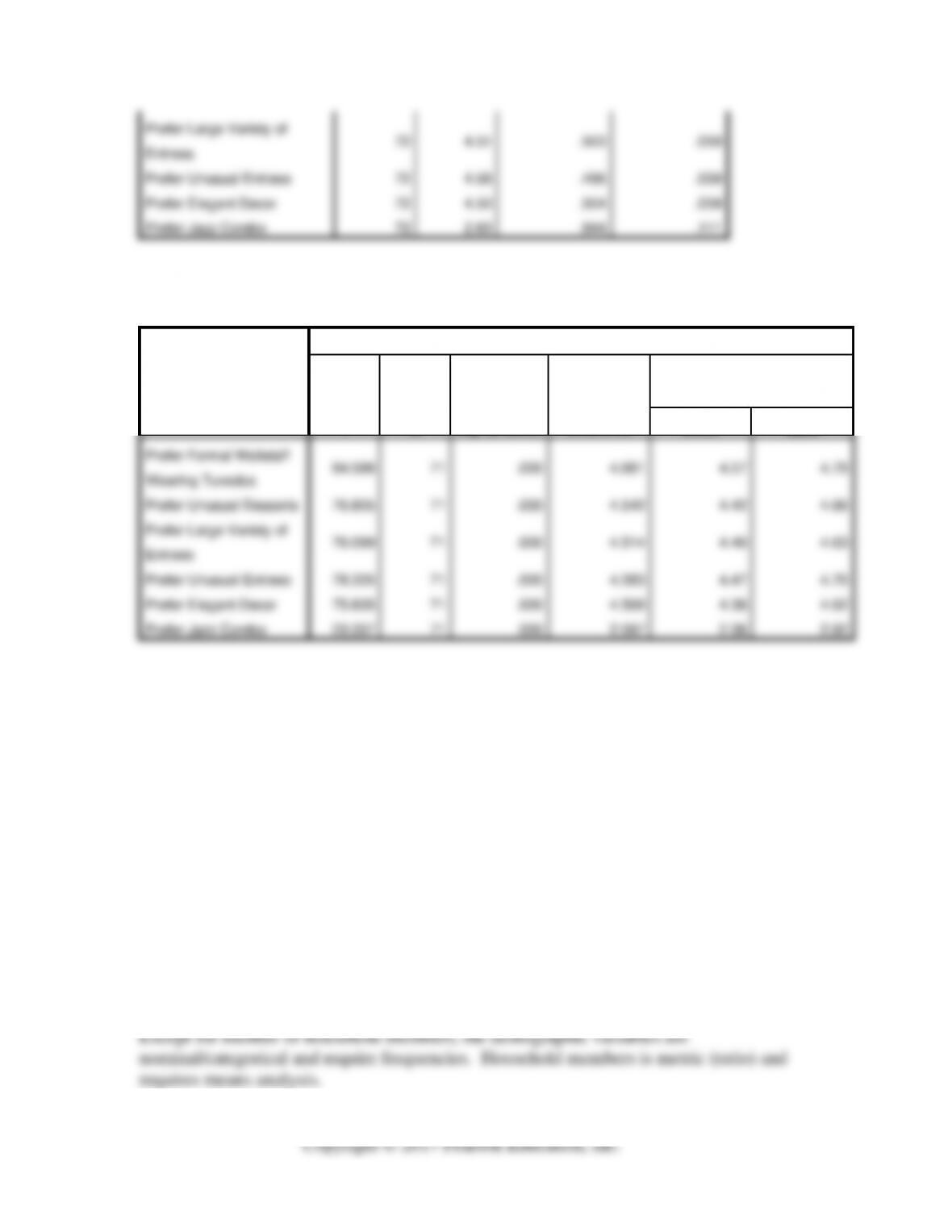
SOMEWHAT PREFER IS A 4 ON THE 5-POINT SCALE, SO TEST THE
HYPOTHESIS THAT THE AVERAGE IS 4. HIS HYPOTHESES OF “SOMEWHAT
PREFER” ARE ALL NOT SUPPORTED. HOWEVER, MANY OF THE AVERAGES
ARE GREATER THAN 4, SO THE PRECISE HYPOTHESIS IS NOT SUPPORTED.
PERFORM CONFIDENCE INTERVALS, AND IT IS FUND THAT ALL BUT JAZZ
COMBO ARE PREFERRED IN A RANGE BETWEEN SOMEWHAT AND VERY
STRONGLY PREFER.
One-Sample Statistics
N
Mean
Std. Deviation
Std. Error Mean
Prefer Formal Waitstaff
Wearing Tuxedos
72
4.68
.470
.055
Prefer Unusual Desserts
72
4.54
.502
.059
Prefer Large Variety of
Entrees
72
4.51
.503
.059
Prefer Unusual Entrees
72
4.58
.496
.059
Prefer Elegant Decor
72
4.50
.504
.059
Prefer Jazz Combo
72
2.60
.944
.111
One-Sample Test
Test Value = 0
t
df
Sig. (2-tailed)
Mean
Difference
95% Confidence Interval of the
Difference
Lower
Upper
Prefer Formal Waitstaff
Wearing Tuxedos
84.586
71
.000
4.681
4.57
4.79
Prefer Unusual Desserts
76.805
71
.000
4.542
4.42
4.66
Prefer Large Variety of
Entrees
76.099
71
.000
4.514
4.40
4.63
Prefer Unusual Entrees
78.335
71
.000
4.583
4.47
4.70
Prefer Elegant Decor
75.835
71
.000
4.500
4.38
4.62
Prefer Jazz Combo
23.337
71
.000
2.597
2.38
2.82
Case 15.3 Auto Concepts Descriptive and Inference Analysis
Case Objective
Students must use the SPSS data set pertaining to integrated case, Advanced Automobile
Concepts, determine the scaling assumptions underlying each question, run the proper
descriptive analysis, and interpret the findings.
Answers to Case Questions
The proper SPSS output follows each question.
1. What is the demographic composition of the sample?
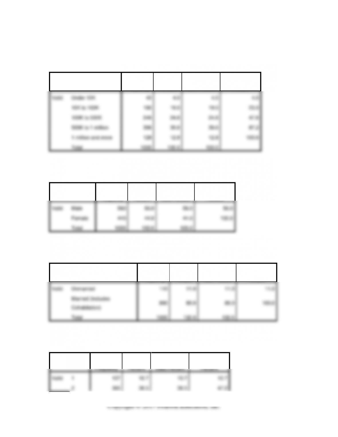
Frequencies
Size of home town or city
Frequency
Percent
Valid Percent
Cumulative
Percent
Valid
Under 10K
40
4.0
4.0
4.0
10K to 100K
190
19.0
19.0
23.0
100K to 500K
246
24.6
24.6
47.6
500K to 1 million
396
39.6
39.6
87.2
1 million and more
128
12.8
12.8
100.0
Total
1000
100.0
100.0
Gender
Frequency
Percent
Valid Percent
Cumulative
Percent
Valid
Male
560
56.0
56.0
56.0
Female
440
44.0
44.0
100.0
Total
1000
100.0
100.0
Marital status
Frequency
Percent
Valid Percent
Cumulative
Percent
Valid
Unmarried
110
11.0
11.0
11.0
Married (Includes
Cohabitation)
890
89.0
89.0
100.0
Total
1000
100.0
100.0
Number of people in household
Frequency
Percent
Valid Percent
Cumulative
Percent
Valid
1
107
10.7
10.7
10.7
3
386
38.6
38.6
85.8
4
106
10.6
10.6
96.4
5
30
3.0
3.0
99.4
6
6
.6
.6
100.0
Total
1000
100.0
100.0
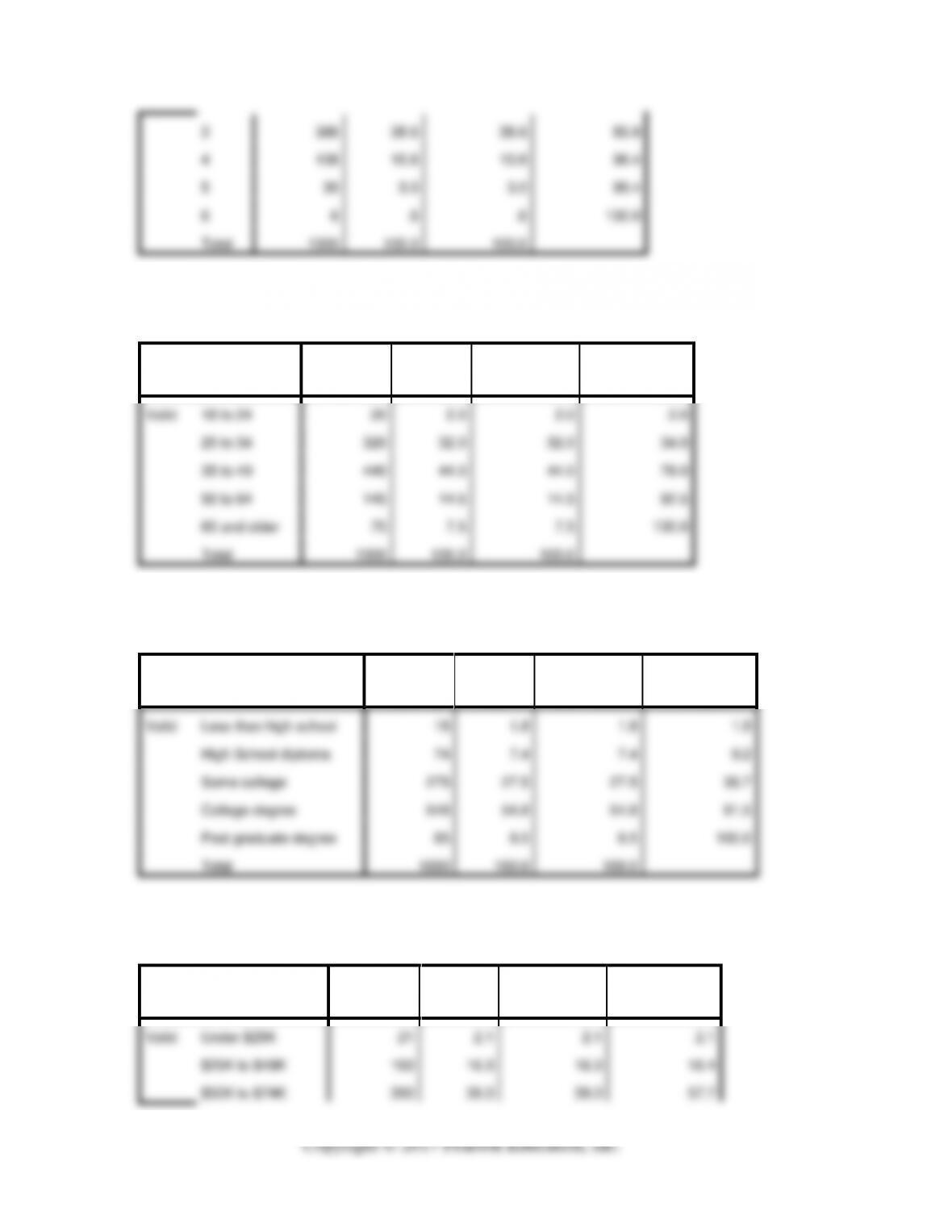
Age category
Frequency
Percent
Valid Percent
Cumulative
Percent
Valid
18 to 24
20
2.0
2.0
2.0
25 to 34
320
32.0
32.0
34.0
35 to 49
440
44.0
44.0
78.0
50 to 64
145
14.5
14.5
92.5
65 and older
75
7.5
7.5
100.0
Total
1000
100.0
100.0
Level of education
Frequency
Percent
Valid Percent
Cumulative
Percent
Valid
Less than high school
18
1.8
1.8
1.8
High School diploma
74
7.4
7.4
9.2
Some college
275
27.5
27.5
36.7
College degree
548
54.8
54.8
91.5
Post graduate degree
85
8.5
8.5
100.0
Total
1000
100.0
100.0
Income category
Frequency
Percent
Valid Percent
Cumulative
Percent
Valid
Under $25K
21
2.1
2.1
2.1
$25K to $49K
163
16.3
16.3
18.4
$75K to $125K
332
33.2
33.2
90.9
$125K and more
91
9.1
9.1
100.0
Total
1000
100.0
100.0
Dwelling type
Frequency
Percent
Valid Percent
Cumulative
Percent
Valid
Single family
319
31.9
31.9
31.9
Multiple family
377
37.7
37.7
69.6
Condominium/Townhouse
219
21.9
21.9
91.5
Moble home
85
8.5
8.5
100.0
Total
1000
100.0
100.0
Descriptives
Descriptive Statistics
N
Minimum
Maximum
Mean
Std. Deviation
Number of people in
household
1000
1
6
2.61
.958
Valid N (listwise)
1000
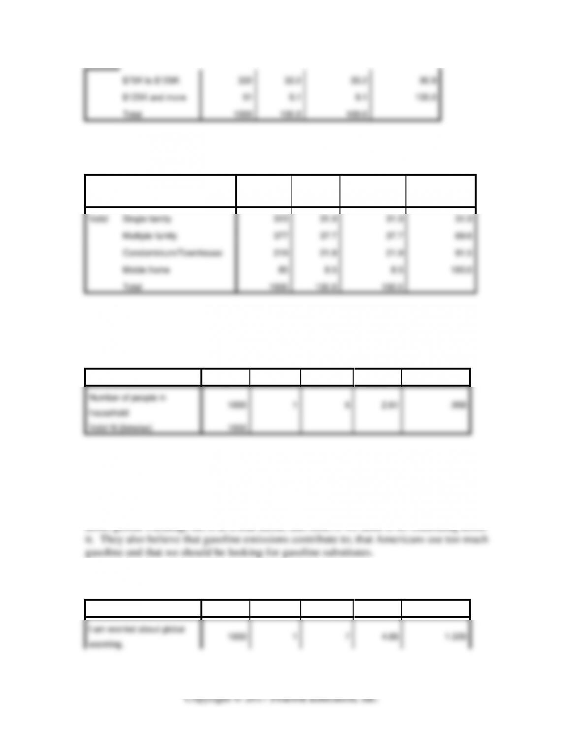
2. How do respondents feel about (1) global warming and (2) gasoline emissions?
Both sets are metric (interval scales), so use Descriptives with means. They are worried
about global warming; see it as a real threat, and believe we need to do something about
Descriptive Statistics
N
Minimum
Maximum
Mean
Std. Deviation
I am worried about global
warming.
1000
1
7
4.88
1.329
Gasoline emissions
contribute to global
warming.
1000
1
7
4.62
1.697
Valid N (listwise)
1000
THE AVERAGES ARE ABOUT 5, OR “AGREE” ON THE 7-POINT SCALE.
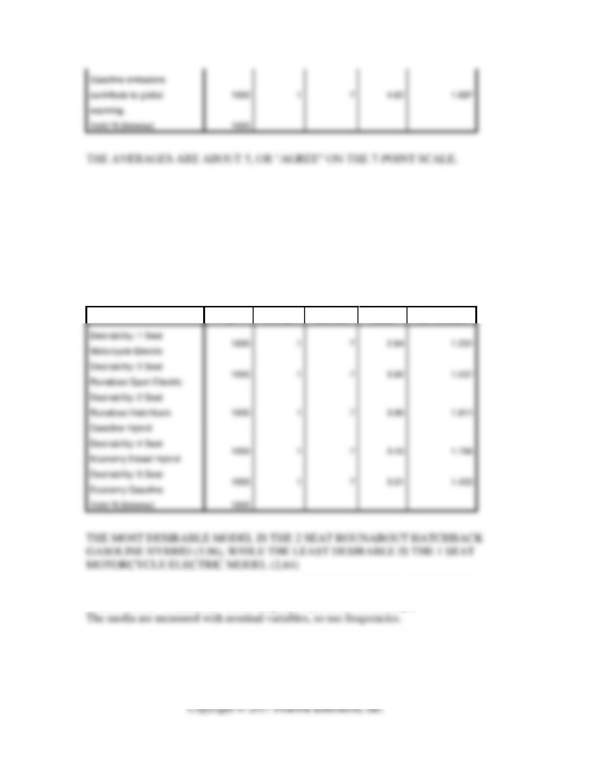
3. What type of automobile model is the most desirable to people in the sample? What
type is the least desirable?
Interval scale requires means. The standard size, synthetic fuel is most popular, and the 1
seat hybrid is the least popular.
Descriptive Statistics
N
Minimum
Maximum
Mean
Std. Deviation
Desirability: 1 Seat
Motorcycle Electric
1000
1
7
2.64
1.231
Desirability: 2 Seat
Runabout Sport Electric
1000
1
7
3.92
1.537
Desirability: 2 Seat
Runabout Hatchback
Gasoline Hybrid
1000
1
7
3.96
1.911
Desirability: 4 Seat
Economy Diesel Hybrid
1000
1
7
3.46
1.768
Desirability: 5 Seat
Economy Gasoline
1000
1
7
3.21
1.453
Valid N (listwise)
1000
THE MOST DESIRABLE MODEL IS THE 2 SEAT ROUNABOUT HATCHBACK
GASOLINE HYBRID (3.96), WHILE THE LEAST DESIRABLE IS THE 1 SEAT
MOTORCYCLE ELECTRIC MODEL (2.64)
4. Describe the “traditional” media usage of respondents in the sample.
Favorite television show type
Frequency
Percent
Valid Percent
Cumulative
Percent
Valid
Comedy
70
7.0
7.0
7.0
Drama
176
17.6
17.6
24.6
Movies/Miniseries
195
19.5
19.5
44.1
Documentary
254
25.4
25.4
69.5
Reality
76
7.6
7.6
77.1
Science Fiction
71
7.1
7.1
84.2
Sports
158
15.8
15.8
100.0
Total
1000
100.0
100.0
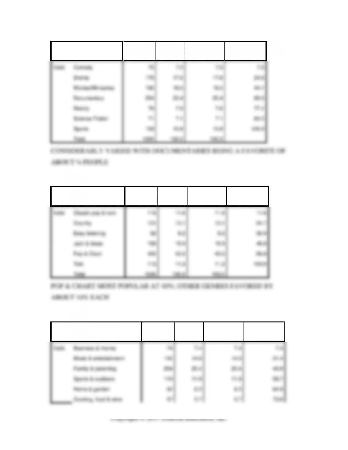
CONSIDERABLY VARIED WITH DOCUMENTARIES BEING A FAVORITE OF
ABOUT ¼ PEOPLE
Favorite radio genre
Frequency
Percent
Valid Percent
Cumulative
Percent
Valid
Classic pop & rock
116
11.6
11.6
11.6
Country
131
13.1
13.1
24.7
Easy listening
82
8.2
8.2
32.9
Jazz & blues
159
15.9
15.9
48.8
Pop & Chart
400
40.0
40.0
88.8
Talk
112
11.2
11.2
100.0
Total
1000
100.0
100.0
POP & CHART MOST POPULAR AT 40%; OTHER GENRES FAVORED BY
ABOUT 10% EACH
Favorite magazine type
Frequency
Percent
Valid Percent
Cumulative
Percent
Valid
Business & money
74
7.4
7.4
7.4
Music & entertainment
140
14.0
14.0
21.4
Family & parenting
254
25.4
25.4
46.8
Sports & outdoors
119
11.9
11.9
58.7
Home & garden
62
6.2
6.2
64.9
Valid N (listwise)
1000
Trucks, Cars & Motorcycles
41
4.1
4.1
74.7
News, politics & current
events
253
25.3
25.3
100.0
Total
1000
100.0
100.0
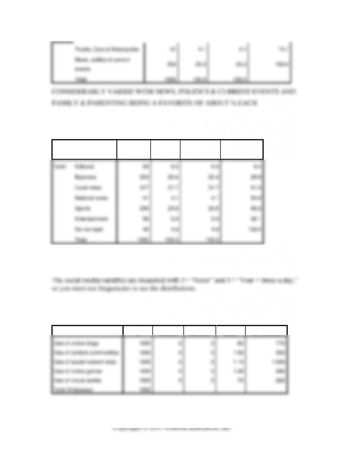
CONSIDERABLY VARIED WITH NEWS, POLITICS & CURRENT EVENTS AND
FAMILY & PARENTING BEING A FAVORITE OF ABOUT ¼ EACH
Favorite local newspaper section
Frequency
Percent
Valid Percent
Cumulative
Percent
Valid
Editorial
94
9.4
9.4
9.4
Business
204
20.4
20.4
29.8
Local news
317
31.7
31.7
61.5
National news
41
4.1
4.1
65.6
Sports
236
23.6
23.6
89.2
Entertainment
59
5.9
5.9
95.1
Do not read
49
4.9
4.9
100.0
Total
1000
100.0
100.0
5. Describe the social media usage of the respondents in the sample.
Descriptive Statistics
N
Minimum
Maximum
Mean
Std. Deviation
Use of online blogs
1000
0
3
.59
.776
Use of content communities
1000
0
3
1.06
.933
Use of social network sites
1000
0
3
1.15
1.005
Use of online games
1000
0
3
1.08
.895
Use of virtual worlds
1000
0
3
.76
.822
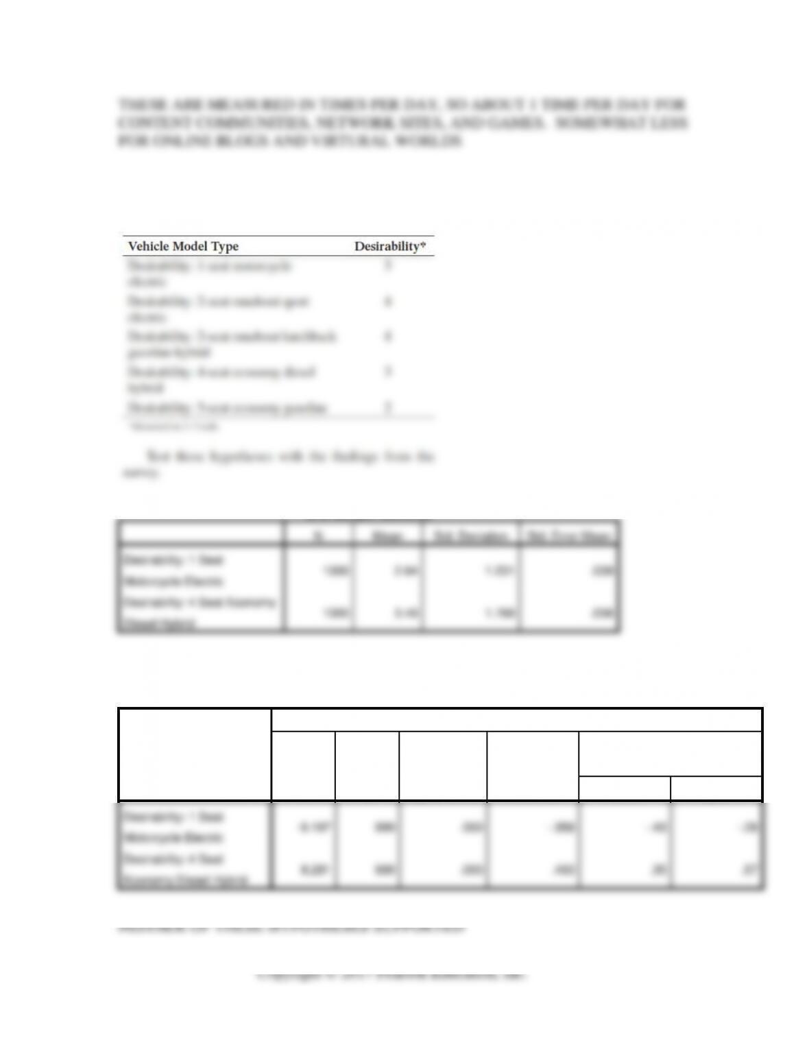
6. The Auto Concepts principals believe that the desirability on the part of the American
public for each of the automobile models under consideration is the following:
One-Sample Statistics
N
Mean
Std. Deviation
Std. Error Mean
Desirability: 1 Seat
Motorcycle Electric
1000
2.64
1.231
.039
Desirability: 4 Seat Economy
Diesel Hybrid
1000
3.46
1.768
.056
One-Sample Test
Test Value = 3
t
df
Sig. (2-tailed)
Mean
Difference
95% Confidence Interval of the
Difference
Lower
Upper
Desirability: 1 Seat
Motorcycle Electric
-9.197
999
.000
-.358
-.43
-.28
Desirability: 4 Seat
Economy Diesel Hybrid
8.281
999
.000
.463
.35
.57
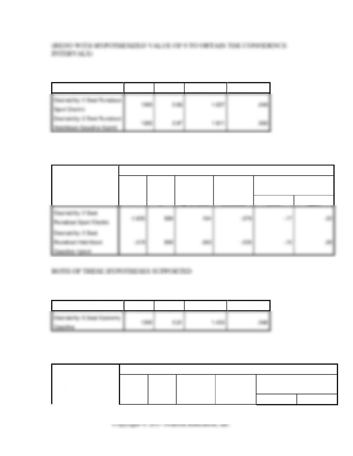
One-Sample Statistics
N
Mean
Std. Deviation
Std. Error Mean
Desirability: 2 Seat Runabout
Sport Electric
1000
3.92
1.537
.049
Desirability: 2 Seat Runabout
Hatchback Gasoline Hybrid
1000
3.97
1.911
.060
One-Sample Test
Test Value = 4
t
df
Sig. (2-tailed)
Mean
Difference
95% Confidence Interval of the
Difference
Lower
Upper
Desirability: 2 Seat
Runabout Sport Electric
-1.626
999
.104
-.079
-.17
.02
Desirability: 2 Seat
Runabout Hatchback
Gasoline Hybrid
-.579
999
.563
-.035
-.15
.08
One-Sample Statistics
N
Mean
Std. Deviation
Std. Error Mean
Desirability: 5 Seat Economy
Gasoline
1000
3.21
1.453
.046
One-Sample Test
Test Value = 2
t
df
Sig. (2-tailed)
Mean
Difference
95% Confidence Interval of the
Difference
Lower
Upper
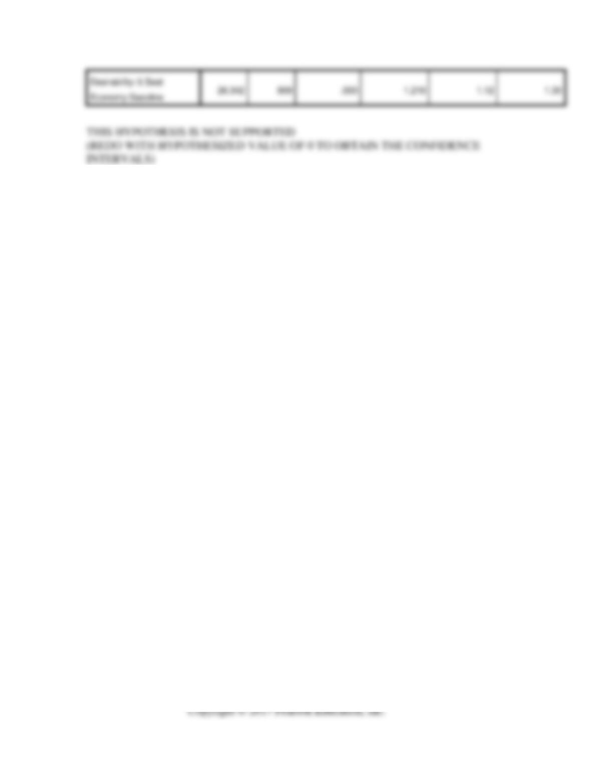
Desirability: 5 Seat
Economy Gasoline
26.342
999
.000
1.210
1.12
1.30
THIS HYPOTHESIS IS NOT SUPPORTED
(REDO WITH HYPOTHESIZED VALUE OF 0 TO OBTAIN THE CONFIDENCE
INTERVALS)