
CHAPTER 12
USING DESCRIPTIVE ANALYSIS, PERFORMING POPULATION
ESTIMATES, AND TESTING HYPOTHESES
LEARNING OBJECTIVES
In this chapter you will learn:
12-1 What the different types of statistical analyses used in marketing research are
12-2 Descriptive analysis and how to do it
12-3 When to use a particular descriptive analysis measure
12-4 How to perform descriptive analyses with SPSS
12-5 How to report descriptive statistics to clients
12-6 The difference between sample statistics and population parameters
12-7 How to estimate the population percent or mean with a confidence interval
12-8 How to obtain confidence intervals with SPSS
12-9 How to report confidence intervals to clients
12-10 What hypothesis tests are and how to perform them
12-11 How to report hypothesis tests to clients
CHAPTER OUTLINE
Types of Statistical Analyses Used in Marketing Research
• Descriptive Analysis
• Inference Analysis
• Difference Analysis
• Association Analysis
• Relationships Analysis
Understanding Descriptive Analysis
• Measures of Central Tendency: Summarizing the “Typical” Respondent
o Mode

o Median
o Mean
• Measures of Variability: Visualizing the Diversity of Respondents
o Frequency and Percentage Distribution
o Range
o Standard Deviation
When to Use a Particular Descriptive Measure
The Auto concepts Survey: Obtaining Descriptive Statistics with SPSS
• Integrated Case
• Use SPSS To Open UP and Use The Auto concepts Dataset
• Obtaining a Frequency Distribution and the Mode with SPSS
• Finding the Median with SPSS
• Finding the Mean, Range, and Standard Deviation with SPSS
Reporting Descriptive Statistics to Clients
• Reporting Scale Data (Ration and Interval Scales)
• Reporting Nominal or Categorical Data
Statistical Inference: Sample Statistics and Population Parameters
Parameter Estimation: Estimating the Population Percent or Mean
• Sample Statistic
• Standard Error
• Confidence Intervals
• How to Interpret an Estimated Population Mean or Percentage Range
The Auto Concepts Survey: How to Obtain and Use a Confidence Interval for a
Mean with SPSS
• Obtaining and Interpreting a Confidence Interval for a Mean
• Using a Confidence Interval to Estimate Market Potential
Reporting Confidence Intervals to Clients
Hypothesis Tests
• Test of the Hypothesized Population Parameter Value
• Auto Concepts: How to Use SPSS to Test a Hypothesis for a Mean
Reporting Hypothesis Tests to Clients
KEY TERMS
Data analysis Descriptive analysis

Inference analysis Difference analysis
Association analysis Relationship analysis
Measures of central tendency Mode
Median Mean
Measures of variability Frequency distribution
Percentage distribution Range
Standard deviation Variance
Statistics Parameters
Inference Statistical inference
Parameter estimate Hypothesis testing
Parameter estimation
Standard error Confidence intervals
Most commonly used level of confidence Hypothesis
Hypothesis test Hypothesized population parameter
Sampling distribution concept
TEACHING SUGGESTIONS
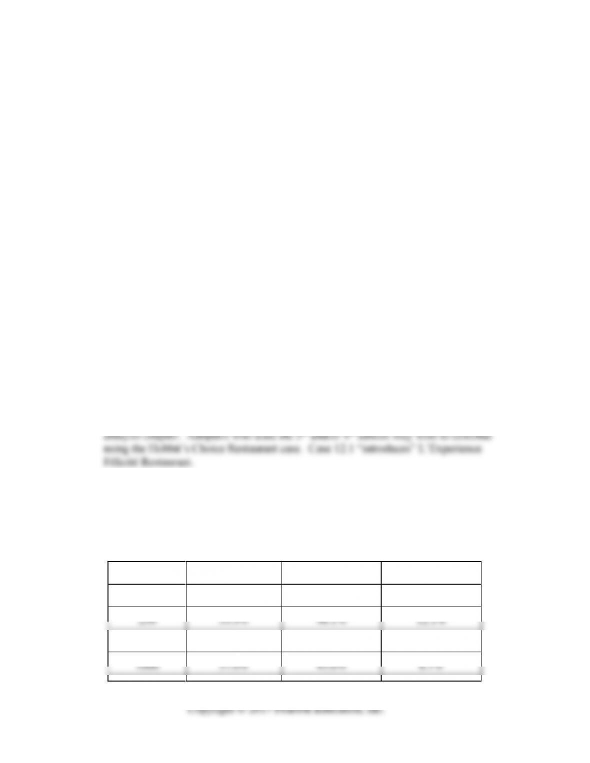
1. Chapter 12 describes descriptive analysis in detail. The four other types of analysis—
inferential analyses, differences analysis, associative analysis, and predictive
analysis—are described very briefly simply to provide an overview. Each type is
described in detail in the following chapters. For chapter 12, students need to know
only the definitions and basic purpose of these analysis types. Table 12.1 is a concise
summary of the various types of analysis, plus it indicates subsequent chapters that
take up each analysis type. Instructors may want to refer to this table as a preview of
what topics will be covered in coming classes.
2. Students can fall into the assumption that because SPSS allows them to define
variables as nominal, ordinal, or scale, it “knows” the scaling assumptions of the
variables and therefore will perform the correct descriptive analysis. This assumption
is not true as the only relevance of the measurement indication is in SPSS chart
procedures where nominal and ordinal variables are treated as categorical.
3. The use of descriptive statistics can be illustrated effectively by using a research
report. Make PowerPoint presentation files or Word files of the questionnaire used in
the study, and have students identify the scaling assumptions and appropriate
descriptive statistics for various questions. Then show the tables in the report that
communicate the findings. With a multimedia teaching platform, instructors can
perform the descriptive statistics with SPSS, illustrating both the cursor movements
and SPSS output.
4. Instructors who want a different data set or who want to have students learn firsthand
how to build an SPSS data set might consider this suggestion. Have the class identify
a topic of interest pertaining to the university and design a self-administered
questionnaire. Design the SPSS template for data entry by entering in variable names
and value labels. Distribute the SPSS template file to students. Each student should
gather a set number of questionnaires and enter them into the SPSS template file and
save it as a unique name (such as lastname.sav). The files can be merged into a
master SPSS data file by using the “merge files” command on a master version of
SPSS. Note: The merge files command is not available on the student version of
SPSS. By spreading the data collection and data entry work across the class, a large
data set can be obtained quickly and efficiently.
5. Our new integrated case is AutoConcepts, and we have a complete SPSS data set for
examples in the text as well as exercises and an integrated case analysis task for each
6. The effect of sample size on a confidence interval can be demonstrated with a simple
spreadsheet program such as Excel or Lotus 1-2-3. Let’s assume that p has been
found to be 40%, what would be the confidence intervals under successively larger
sample sizes? The following table is a spreadsheet-like comparison for 95%
confidence intervals.
Sample Size
Lower Limit
Upper Limit
Range
100
30.4%
49.6%
19.2%
250
33.9%
46.1%
12.1%
500
35.7%
44.3%
8.6%
1000
37.0%
43.0%
6.1%
1500
37.5%
42.5%
5.0%
2000
37.9%
42.1%
4.3%
7. Some textbooks, particularly statistics textbooks, explicitly state the alternative
hypothesis. We do not do so in our textbook, but we have included a Marketing
Research Insight on “What Is an Alternative Hypothesis?” Instructors who believe
8. With SPSS for Windows available to them, student may not appreciate doing hand
calculations of confidence intervals or hypothesis tests. These calculations are more
9. There are a few, but not many, hand calculation end-of-chapter questions. It may be
beneficial to devote part of a class to in-class exercises where students calculate
confidence intervals or test hypotheses using the end-of-chapter questions or
questions generated by the instructor. Ask students to bring their hand calculators.
Having each student work independently in a class setting and providing the step-by-
step calculations will force students to use the formulas correctly.
ACTIVE LEARNING EXERCISES
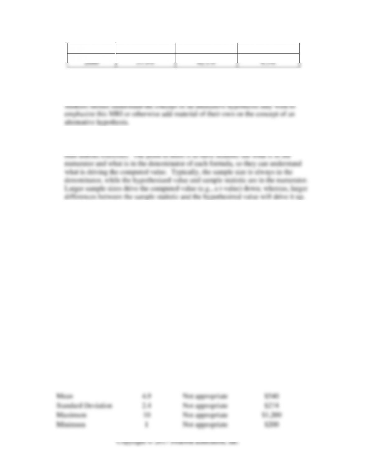
Compute Measures of Central Tendency and Variability
This exercise provides a dataset and requires students to compute the appropriate
measures of central tendency and variability. The answers are provided below the data
table.
For how many
years have you
owned your gas
grill?
Where did you
purchase your
gas grill?
About how
much did your
pay for your
gas grill?
Median
4.5
Not appropriate
$450
Mode
4
Not appropriate
$400
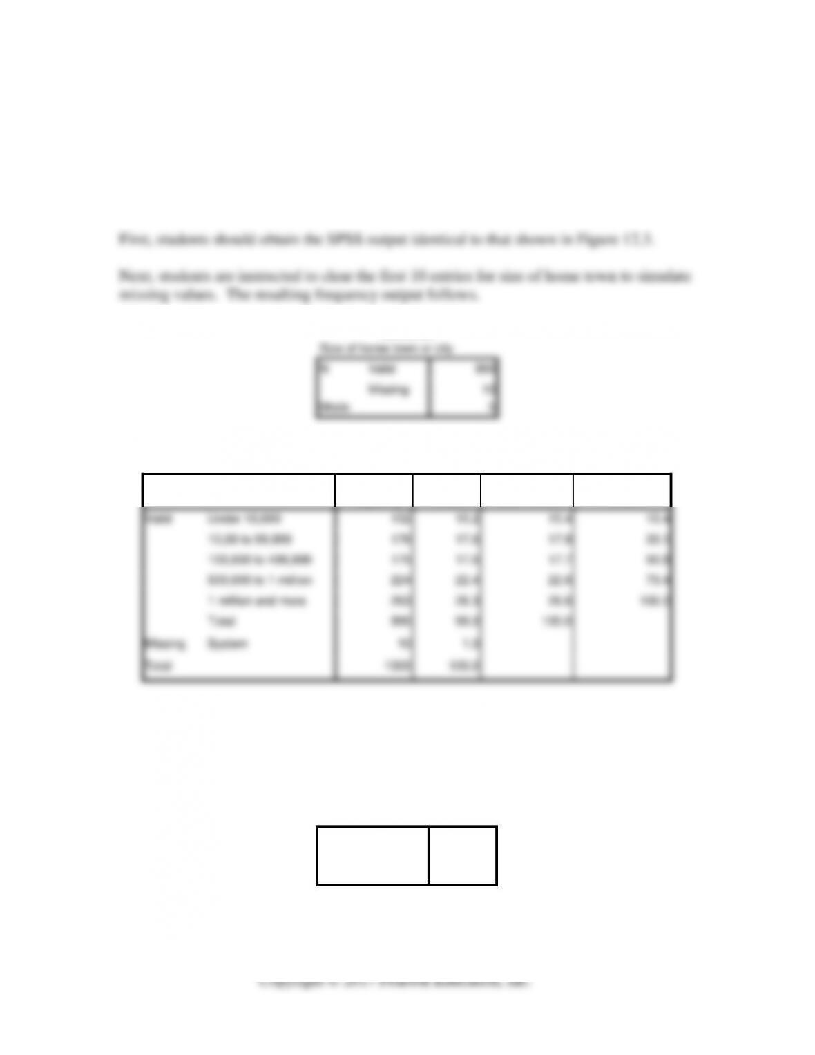
Use your SPSS Auto Concept data set to compute the frequency distribution and
percentage distribution…
Statistics
Size of home town or city
N
Valid
990
Missing
10
Mode
5
Size of home town or city
Frequency
Percent
Valid Percent
Cumulative
Percent
Valid
Under 10,000
152
15.2
15.4
15.4
10,00 to 99,999
176
17.6
17.8
33.1
100,000 to 499,999
175
17.5
17.7
50.8
500,000 to 1 million
224
22.4
22.6
73.4
1 million and more
263
26.3
26.6
100.0
Total
990
99.0
100.0
Missing
System
10
1.0
Total
1000
100.0
Find a Median with SPSS
Students should follow the instructions to obtain the median and the following output.
Statistics
Income category
N
Valid
1000
Missing
0
Median
2.00
Income category
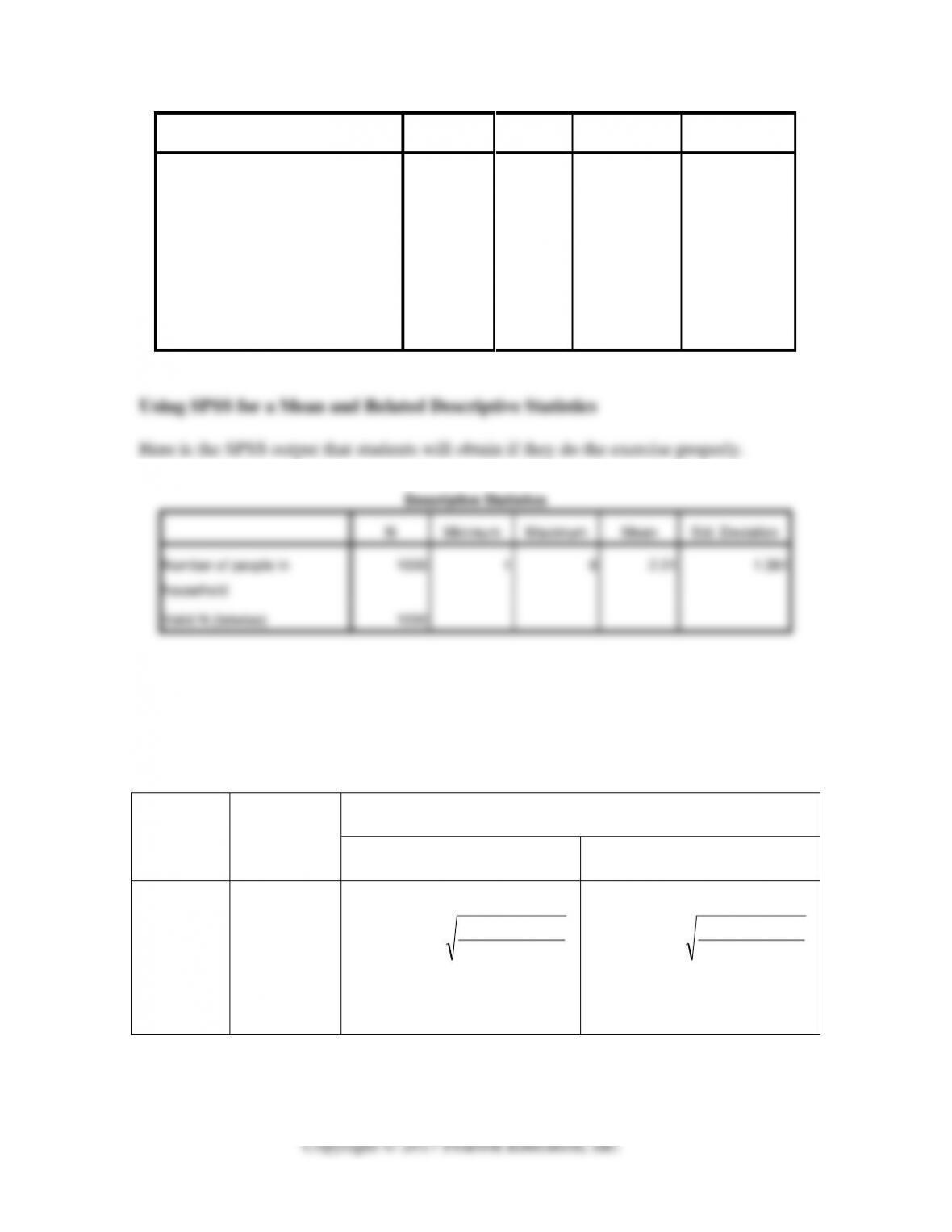
Frequency
Percent
Valid Percent
Cumulative
Percent
Valid
Under $25,000
256
25.6
25.6
25.6
Between $25,000 and
$49,999
343
34.3
34.3
59.9
Between $50,000 and
$74,999
194
19.4
19.4
79.3
Between $75,000 and
$124,999
137
13.7
13.7
93.0
$125,000 and higher
70
7.0
7.0
100.0
Total
1000
100.0
100.0
Descriptive Statistics
N
Minimum
Maximum
Mean
Std. Deviation
Number of people in
household
1000
1
9
2.21
1.381
Valid N (listwise)
1000
Calculate Some Confidence Intervals
This exercise provides students with experience in calculating confidence intervals for
percentages and for a mean. In all cases, the sample size is 1,000, and they are to use the
formulas provided in the chapter.
Question
Sample
Statistic(s)
95% Confidence Interval
Lower boundary
Upper boundary
Have you
heard of
satellite
radio?
50%
responded
“yes”
%4.48
58.150
1000
)50100(*50
*96.150
=
−=
−
−=
p
szp
%6.51
58.150
1000
)50100(*50
*96.150
=
+=
−
+=
p
szp
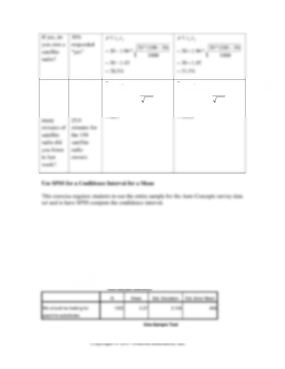
If yes, do
you own a
satellite
radio?
30%
responded
“yes”
%5.28
45.130
1000
)30100(*30
*96.130
=
−=
−
−=
p
szp
%5.31
45.130
1000
)30100(*30
*96.130
=
+=
−
+=
p
szp
If you
own
satellite
radio,
about how
many
minutes of
satellite
radio did
you listen
to last
week?
Average of
100.7
minutes;
standard
deviation of
25.0
minutes for
the 150
satellite
radio
owners
7.96
00.47.100
150
25
*96.17.100
=
−=
−=
x
szx
5.104
00.47.100
150
25
*96.17.100
=
+=
+=
x
szx
Use SPSS for a Confidence Interval for a Mean
This exercise requires students to use the entire sample for the Auto Concepts survey data
set and to have SPSS compute the confidence interval.
You have just learned that the 95% confidence interval for the “Gasoline emissions
contribute to global warming” variable” would include an average of 4.8, with a lower
boundary of 4.68 and an upper boundary of 4.96. What about the statement” We should
be looking for gasoline substitutes”?
To answer this question, you must use SPSS to compute the 95% confidence interval for
the mean of this variable. Use the clickstream identified in Figure 12.7 and use the
annotations in Figure 12.8 to find and interpret your 95% confidence interval for the
public’s opinion on this topic. How do you interpret this finding, and how does this
confidence interval compare to the one we found for “Global warming is a real threat”?
One-Sample Statistics
N
Mean
Std. Deviation
Std. Error Mean
We should be looking for
1000
5.07
2.159
.068
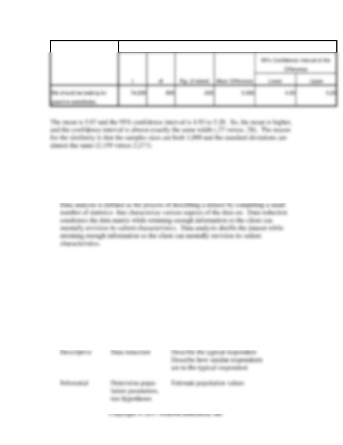
Test Value = 0
t
df
Sig. (2-tailed)
Mean Difference
95% Confidence Interval of the
Difference
Lower
Upper
We should be looking for
gasoline substitutes.
74.209
999
.000
5.066
4.93
5.20
The mean is 5.07 and the 95% confidence interval is 4.93 to 5.20. So, the mean is higher,
and the confidence interval is almost exactly the same width (.27 versus .28). The reason
for the similarity is that the samples sizes are both 1,000 and the standard deviations are
almost the same (2.159 versus 2.277).
ANSWERS TO END-OF-CHAPTER QUESTIONS
1. Indicate what data analysis is and why it is useful.
2. Define and differentiate each of the following:
a. Descriptive analysis
b. Inferential analysis
c. Associative analysis
d. Relationship analysis
e. Differences analysis
Each type of analysis is described in Table 12.1, the pertinent aspects of which are
repeated below.
model
3. What is a measure of central tendency and what does it describe?
4. Explain the concept of variability, and relate how it helps in the description of
responses to a particular question on a questionnaire.
All measures of variability are concerned with depicting the “typical” difference
5. Using examples, illustrate how a frequency distribution (or a percentage distribution)
reveals the variability in responses to a Likert-type question in a life-style study. Use
two extreme examples of much variability and little variability.
6. Indicate what a range is and where it should be used as an indicator of the amount of
dispersion in a sample.
7. With explicit reference to the formula for a standard deviation, show how it measures
how different respondents are from one another.
8. Explain why is the mean an inappropriate measure of central tendency in each of the
following cases:
The scaling assumptions underlying a question determine which statistic is
appropriate. Table 12.2 indicates that the mean should be used when working with
9. For each of the cases in question 8, what is the appropriate central tendency
measure?
Students must identify the scaling assumptions for each measure and indicate the
appropriate central tendency measure.
The correct central tendency measure is listed beneath each case.
a. Gender of respondent (Male or Female)
b. Marital status (Single, Married, Divorced, Separated, Widowed, Other)
c. A taste test where subjects indicate their first, second, and third choices of Miller
Lite, Bud Light, and Coors Silver Bullet
10. In a survey on productivity apps, respondents write in the number of apps they have
installed in the past six months. What measures of central tendency can be used?
Which is the most appropriate and why?
11. If you use the standard deviation as a measure of the variability in a sample, what
statistical assumptions have you implicitly adopted?
12. What essential factors are taken into consideration when statistical inference takes
place?
13. What is meant by “parameter estimation,” and what function does it perform for a
researcher?
and (3) the desired level of confidence (usually 95% or 99%). Parameter estimation
14. How does parameter estimation for a mean differ from that for a percentage?
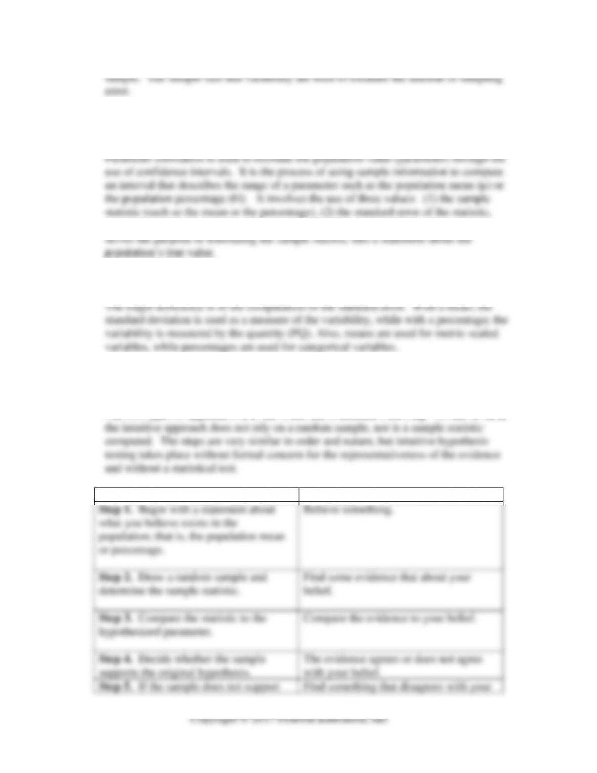
15. List the steps in statistical hypothesis testing and the steps in intuitive hypothesis
testing. How are they similar? How are they different?
The two types of hypothesis tests are listed and contrasted following. As can be seen,
Statistical Hypothesis Steps
Intuitive Hypothesis Steps
Step 1. Begin with a statement about
what you believe exists in the
population; that is, the population mean
or percentage.
Believe something.
Step 2. Draw a random sample and
determine the sample statistic.
Find some evidence that about your
belief.
Step 3. Compare the statistic to the
hypothesized parameter.
Compare the evidence to your belief.
Step 4. Decide whether the sample
supports the original hypothesis.
The evidence agrees or does not agree
with your belief.
Step 5. If the sample does not support
Find something that disagrees with your
the hypothesis, revise the hypothesis to
be consistent with the sample’s statistic.
belief, and now believe something
different.
16. What does it mean when a researcher says that a hypothesis has been supported at
the 95% confidence level?
17. Here are several computation practice exercises to help you identify which formulas
pertain and learn how to perform the necessary calculations. In each case, perform
the necessary calculations and write your answers in the column identified by a
question mark.
a. Determine confidence intervals for each of the following:
48.532.5
08.4.5
250
5.0
58.24.5
−=
=
x
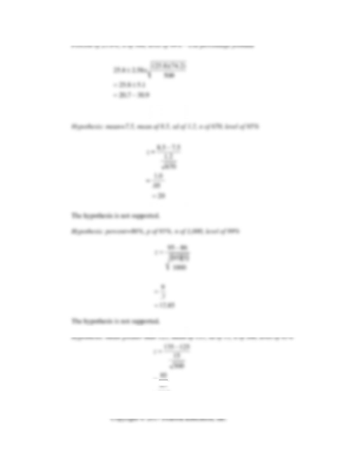
b. Test the hypothesis and interpret your findings.
9.307.20
1.58.25
500
)2.74)(8.25(
58.28.25
−=
=
x
9.14
67.
10
500
15
125135
=
=
−
=
z
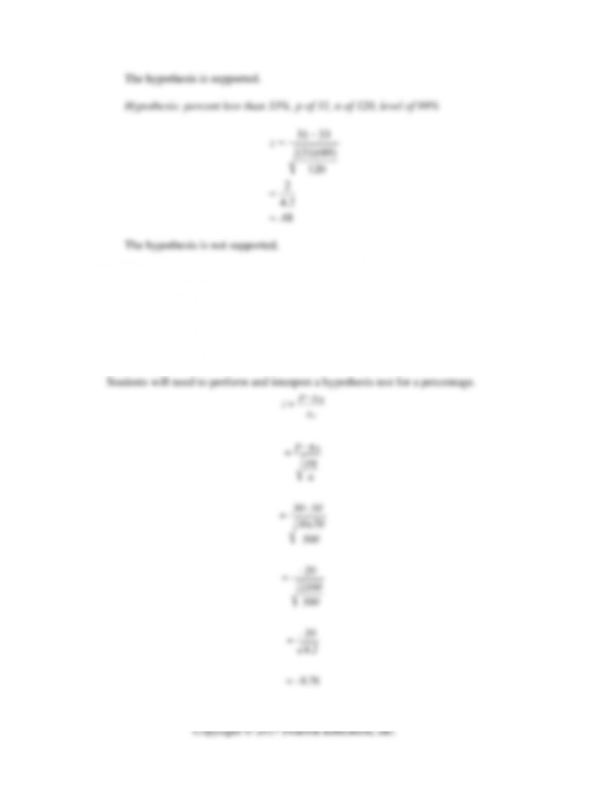
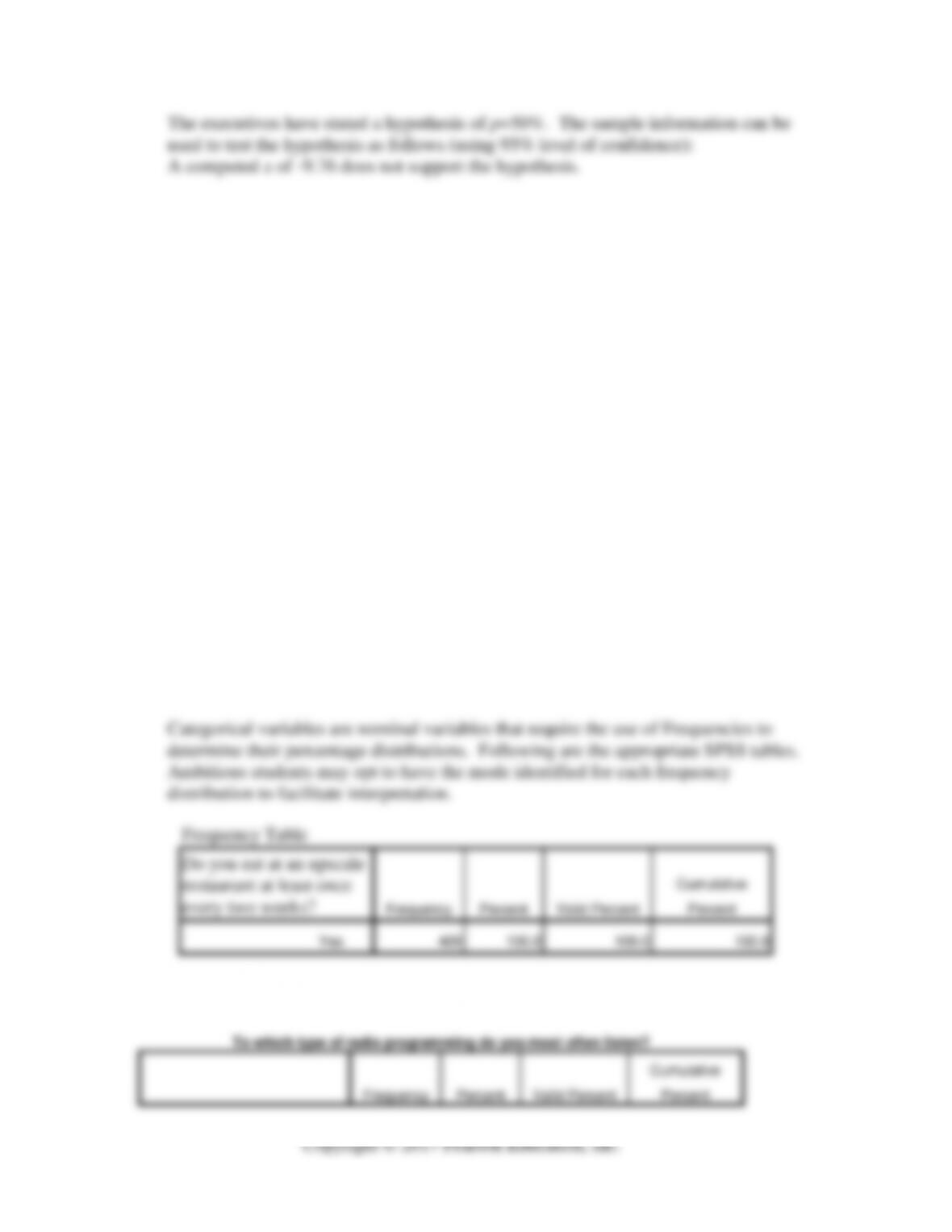
18. Alamo Rent-A-Car executives believe that Alamo accounts for about 50% of all
Cadillacs that are rented. To test this belief, a researcher randomly identifies 20
major airports with on-site rental car lots. Observers are sent to each location and
instructed to record the number of rental-company Cadillacs observed in a four-hour
period. About 500 are observed, and 30% are observed being returned to Alamo
Rent-A-Car. What are the implications of this finding for the Alamo executives’
belief?
CASE SOLUTIONS
Case 12.1 L’Experience Félicité Restaurant Survey Descriptive and Inference
Analysis
Case Objective
Students must use the SPSS data set pertaining to L’Experience Félicité Restaurant case
(This was the integrated case in the previous edition of the textbook), determine the
scaling assumptions underlying each question, run the proper descriptive analysis, and
interpret the findings.
Answers to Case Questions
A convenient way to identify the response codes used in this data set is to open the SPSS
file in SPSS and use the Utilities-Variables command sequence. This command will
provide a window where each variable’s label, value codes, and value labels can be seen.
. The “measure” aspect of each variable has been identified as “nominal” or “scale,” with
“scale” pertaining to interval or ratio scaling assumptions.
1. Determine what variables are categorical (either nominal or ordinal scales), perform
the appropriate descriptive analysis, and interpret it.
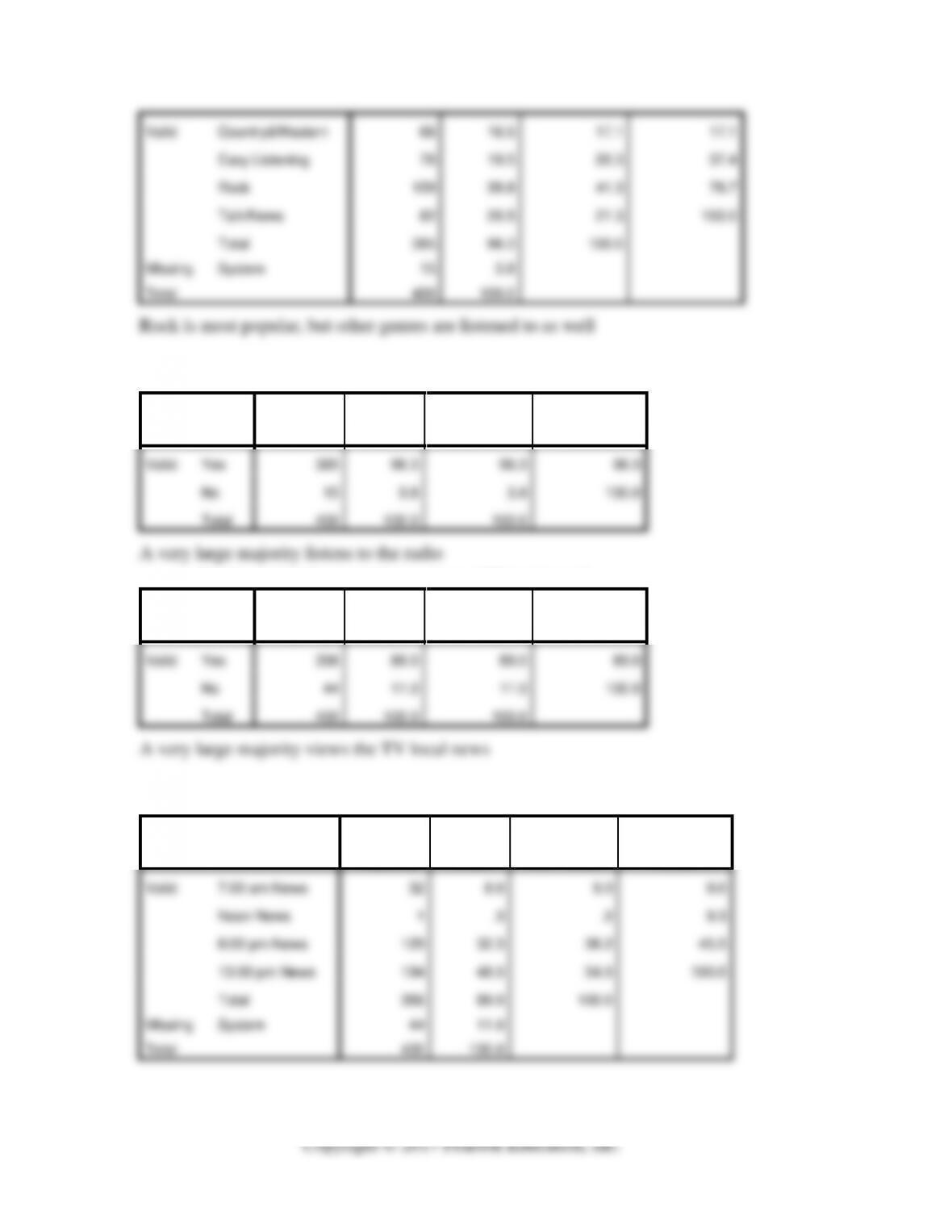
Valid
Country&Western
66
16.5
17.1
17.1
Easy Listening
78
19.5
20.3
37.4
Rock
159
39.8
41.3
78.7
Talk/News
82
20.5
21.3
100.0
Total
385
96.3
100.0
Missing
System
15
3.8
Total
400
100.0
Rock is most popular, but other genres are listened to as well
Would you describe yourself as one who listens to the radio?
Frequency
Percent
Valid Percent
Cumulative
Percent
Valid
Yes
385
96.3
96.3
96.3
No
15
3.8
3.8
100.0
Total
400
100.0
100.0
A very large majority listens to the radio
Would you describe yourself as a viewer of TV local news?
Frequency
Percent
Valid Percent
Cumulative
Percent
Valid
Yes
356
89.0
89.0
89.0
No
44
11.0
11.0
100.0
Total
400
100.0
100.0
A very large majority views the TV local news
Which newscast do you watch most frequently?
Frequency
Percent
Valid Percent
Cumulative
Percent
Valid
7:00 am News
32
8.0
9.0
9.0
Noon News
1
.3
.3
9.3
6:00 pm News
129
32.3
36.2
45.5
10:00 pm News
194
48.5
54.5
100.0
Total
356
89.0
100.0
Missing
System
44
11.0
Total
400
100.0
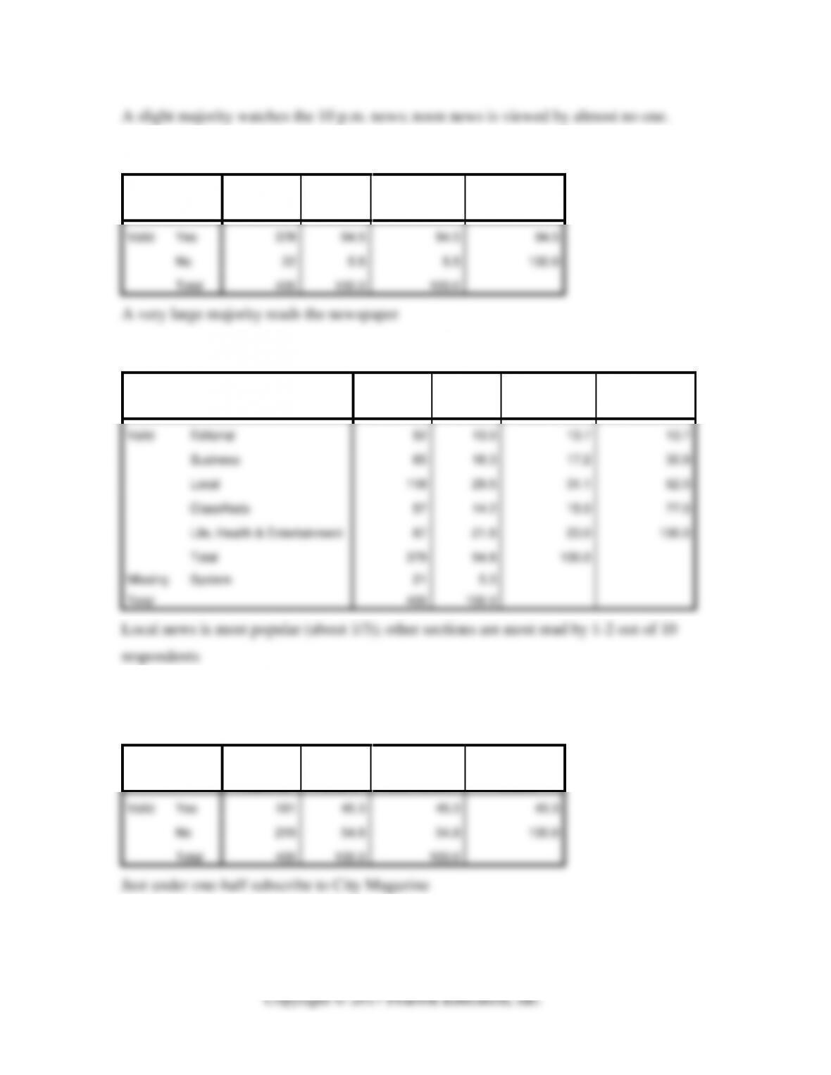
Do you read the newspaper?
Frequency
Percent
Valid Percent
Cumulative
Percent
Valid
Yes
378
94.5
94.5
94.5
No
22
5.5
5.5
100.0
Total
400
100.0
100.0
A very large majority reads the newspaper
Which section of the local newspaper would you say you read most frequently?
Frequency
Percent
Valid Percent
Cumulative
Percent
Valid
Editorial
52
13.0
13.7
13.7
Business
65
16.3
17.2
30.9
Local
118
29.5
31.1
62.0
Classifieds
57
14.2
15.0
77.0
Life, Health & Entertainment
87
21.8
23.0
100.0
Total
379
94.8
100.0
Missing
System
21
5.3
Total
400
100.0
Local news is most popular (about 1/3); other sections are most read by 1-2 out of 10
respondents
Do you subscribe to City Magazine?
Frequency
Percent
Valid Percent
Cumulative
Percent
Valid
Yes
181
45.3
45.3
45.3
No
219
54.8
54.8
100.0
Total
400
100.0
100.0
Just under one-half subscribe to City Magazine
What is your highest level of education?