978-0133872293 Chapter 9 Lecture Note

Unlock access to all the studying documents.

View Full Document

W H AT I S E C O N O M I C S ? 9 9

T h e B i g P i c t u r e

Where we have been:

This chapter, along with Chapter 8, examines the consumer choices that

underlie the law of demand. Budget lines were introduced in Chapter 8 and are

more fully explored in this chapter. This chapter shows how the substitution

e’ect combined with the income e’ect for a normal good always leads to the

downward-sloping demand curve, which was assumed in Chapter 3. The

concept of slope, as explained in Chapter 1 (appendix), is used to show that in

equilibrium the MRS equals the relative price of the goods.

Where we are going:

Chapters 10 and 11 study the theory of the 0rm and the 0rm’s costs, and

Chapters 12 through 15 look at 0rm behavior in di‘erent market structures.

N e w i n t h e Tw e l f t h E d i t i o n

The material in this chapter is similar to the last edition, but the case studies have

been updated. Data has been updated and a new article is used for the

end-of-chapter application. A Worked Problem section has been added. The

Worked Problem presents information about Wendy, who consumes 10 sugary

drinks and 4 smoothies. The government taxes the sugary drinks, changing their

price, and simultaneously changes the income tax, changing Wendy’s income.

The Worked Problem then asks the students to calculate Wendy’s budget, Wendy’s

opportunity cost of a sugary drink, Wendy’s new consumption, and the change in

Wendy’s welfare. Then the Worked Problem demonstrates to the students how to

use the indi’erence curve-budget line model to answer the questions. To include

the new Worked Problem without lengthening the chapter, some problems have

been removed from the Study Plan Problem and Applications. These problems are

in the MyEconLab and are called Extra Problems.

POSSIBILITES,

PREFERENCES,

AND CHOICES

C h a p t e r

L e c t u r e N o t e s

Possibilities, Preferences, and Choices

 A person’s budget in combination with his or her preferences determines what goods

and services the person consumes.

 Using the budget line and indi’erence curves, economists can predict how changes

in the price of a good or service a’ect the quantity a person demands.

I. Consumption Possibilities

 A household’s consumption choices are

constrained by its income and the prices of

the goods and services available. A

household’s budget line describes the limits

to its consumption choices.

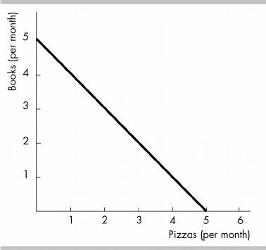
 The 0gure to the right shows a budget line for

a household that buys only pizzas and books.

The household can buy any combination of

pizza and books that lies on or within the

budget line. Combinations that lie beyond the

budget line are una‘ordable.

 Divisible goods can be bought in any quantity

and we can best understand household

choices if we assume all goods are divisible.

 The budget line illustrates a constraint on

choices. Any point on or inside the line can

be purchased. Any point outside the line is una’ordable and cannot be purchased.

Budget Equation

 We can describe the budget line by using a budget equation, which states that

income equals expenditure.

 Calling the price of a book PB, the quantity of books QB, the price of a pizza PP, the

quantity of pizza QP, and income Y, we can write a budget equation as PB  QB + PP

 QP = Y, which can be rearranged into slope-intercept form as QB = Y/PB  (PP/PB)

 QP.

 A household’s real income is the household’s income expressed as a quantity of

goods the household can a’ord to buy. In the 0gure above, in terms of books, the

household’s real income is Y/PB (5 books), which is the vertical intercept of the

budget line.

 A relative price is the price of one good divided by the price of another good. The

magnitude of the slope of the budget line, (PP/PB), is the relative price of a pizza in

terms of a book. A relative price is an opportunity cost, so the relative price of a

pizza in terms of books gives the opportunity cost of a pizza in terms of books

forgone.

 When the price of the good measured along the horizontal axis (pizzas) changes, the

budget line rotates around the vertical intercept. If the price of the good falls, the

budget line rotates outward and becomes ?atter; if the price of the good rises, the

budget line rotates inward and becomes steeper.

 When income changes, the budget line shifts and its slope does not change. If

income increases, the budget line shifts outward; if income decreases, the budget

line shifts inward.

Example: The budget line as a menu. Emphasize that the consumer’s budget line is

like that part of a menu that delineates all a’ordable combinations of food and drinks that

are available to the consumer given a budget.

If you want to push this analogy, have the students assign a price to each of the two goods

and then choose a level of income to be spent on the dinner. Draw the budget line and then

have the students show how a rise in the price of drinks or the price of food would rotate

the budget line and change relative prices. Then have the students help you illustrate how

an increase in income shifts the budget line allowing more food (perhaps dessert) and the

second glass of wine.

II. Preferences and Indi*erence Curves

 A preference map shows how a person

ranks various combinations of goods and

services.

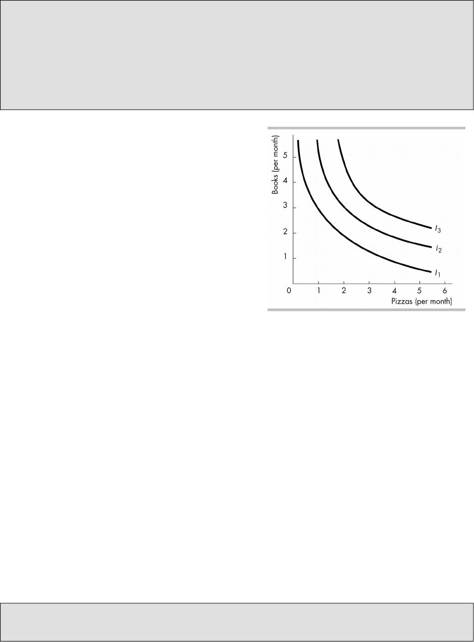
 Indi’erence curves are used to illustrate a

person’s preference map. An

indi*erence curve is a line that shows

combinations of goods among which a

consumer is indierent. The 0gure to the

right shows three of a person’s

indi‘erence curves between pizza and

books.

By construction the consumer is

indi‘erent among all the points on

any particular indi’erence curve.

 The consumer prefers points above

any particular indi’erence curve to

points on the curve. And the consumer prefers points on the indi’erence curve

to points below the curve. In the 0gure, the consumer prefers any point on

indi‘erence curve I2 to any point on I1 and any point on I3 to any point on I2.

Marginal Rate of Substitution

 The marginal rate of substitution (MRS) is the rate at which a person will give up

good y (the good measured on the y-axis) to get an additional unit of good x (the

good measured on the x-axis) and at the same time remaining indi’erent

(remaining on the same indi’erence curve).

 The magnitude of the slope of the indi’erence curve at any point measures the

marginal rate of substitution between the goods. If the indi’erence curve is

steep, the MRS is high; if the indi’erence curve is ?at, the MRS is small.

 The diminishing marginal rate of substitution is the general tendency for a

person to be willing to give up less of good y to get one unit of good x, and at

the same time remain indi‘erent, as the quantity of x increases. This principle

implies that indi’erence curves generally become ?atter moving along them to

the right.

Degree of Substitutability

 The indi‘erence curves between most goods are bowed in, with a diminishing MRS.

 The indi‘erence curves for perfect substitutes are linear, with a constant MRS.

 The indi‘erence curves for perfect complements are L–shaped. Utility increases (the

consumer moves to a higher indi’erence curve) only if the quantity of both goods x

and y increases.

Perfect substitutes or just substitutes? Students will remember discussions of

substitutes and complements in consumption from Chapter 3, and often don’t see how

“perfect” substitutes or complements are any di’erent. Be sure to use examples to show

9 4 C H A P T E R 9

how, even for most goods that are considered substitutes (or complements), the MRS will

still be diminishing. Only when a consumer’s willingness to trade one good for the other is

constant (i.e., MRS is linear) are two goods considered “perfect” substitutes. Similarly, you

may drink cream in your co’ee, implying co’ee and cream are complements, but they’re

not likely to be “perfect” complements. A cup of co’ee without cream may still be better

(increase your utility) than no co’ee at all.

P O S S I B I L I T I E S , P R E F E R E N C E S , A N D C H O I C E S 9 5

III. Predicting Consumer Choices

Best Aordable Choice

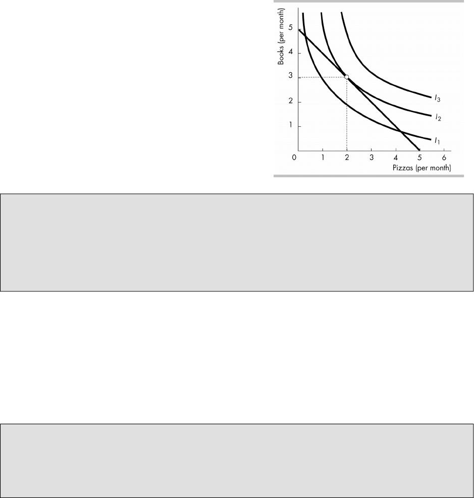
 The consumer will select his or her best

a’ordable point. This point:

 is on the budget line,

 is on the highest attainable

indi‘erence curve,

 has a marginal rate of substitution

between the two goods equal to the

relative price of the two goods.

 The 0gure shows the best a’ordable point,

2 pizzas and 3 books. This combination is

on the budget, and hence is “a’ordable.” It

also is on the highest indi’erence curve so

that the marginal rate of substitution

equals the relative price of the two goods,

and hence the point is “best.”

The meaning of tangency. Emphasize to your students the meaning behind the

tangency point between the indi’erence curve and the budget line. In particular, the

marginal rate of substitution (MRS) shows the consumer’s willingness to give up one good

to get more of the other good. The relative price of the two goods shows what the

consumer must give up one good to get more of the other good. When a consumer equates

the marginal rate of substitution (MRS) to the relative price ratio, the consumer is just

willing to give up what he or she must give up, and there are no unrealized gains from

substituting one good for another.

A Change In Price

 The price e*ect shows how a change in the price of a good a’ects the quantity

consumed of that good.

 When the price of the good on the x-axis falls, the budget line rotates around the

y-axis intercept and becomes ?atter. The person moves to a new consumption point.

The new consumption bundle satis0es all three properties: It is on the new budget

line, it is on the highest attainable indi‘erence curve, and the MRS equals the slope

of the new budget line.

 When the price of a good changes, tracking the change in the quantity of the good

consumed reveals the demand curve for that good.

The Economics in Action case study considers how the best a’ordable combination of

movies and DVD rentals has changed over time, largely due to changes in the DVD rental

market. The case study points out that a major factor leading to these changes is a fall in

the price of renting a DVD (thanks to Redbox) that allowed people to rent more DVDs and

see more movies. Have students illustrate this result for themselves, shifting the budget

line between movies and DVDs and seeing what the new equilibrium might look like.

A Change In Income

 The income e*ect shows how a change in income a’ects the buying plans of

consumers.

 When the price of the goods remains constant, a change in income shifts the budget

line. This shift changes which indi’erence curve is highest attainable indi‘erence

curve. The person moves to a new consumption point. The new consumption bundle

satis0es all three properties: it is on the new budget line; it is on the highest

attainable indi‘erence curve; and the MRS equals the slope of the new budget line.

9 6 C H A P T E R 9

 A change in income shifts the demand curve, because a di’erent quantity is

consumed at the same prices.

 If income rises and more is consumed at each price (or if income falls and less is

consumed at each price) the good is a normal good.

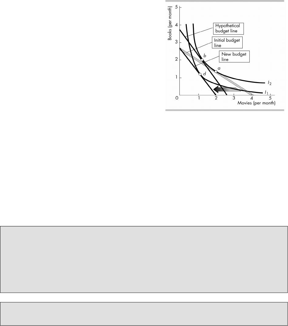
Substitution Eect and Income Eect

 For a normal good, a rise in price always decreases the quantity consumed. This

result is shown by breaking the price e’ect into two parts, as illustrated in the 0gure

in which the price of movies rise:

 The substitution e*ect is the e’ect

of a change in price on the quantity

bought when the consumer

(hypothetically) remains indi‘erent

between the original situation and the

new one. The substitution e’ect is

showing by moving the new budget

line (with its new slope) so that it is

tangent to the initial indi’erence

curve. This procedure creates a

(hypothetical) new best a’ordable

point using the initial indi’erence

curve and the hypothetical budget

line. Comparing the initial best

a’ordable point to this new one

captures the substitution e’ect. In the

0gure this compares point a to point b. The substitution e’ect of a rise in price

always leads to a decrease in the quantity consumed.

 The income e*ect is the e’ect on the quantity bought of a change in income

suKcient to shift the hypothetical budget line used to measure the substitution

e’ect, so that it is the same as the actual new budget line. This process is the

movement from point b to point d in the 0gure. For a rise in price, this change

requires a decrease in income. For a normal good, the decrease in income

decreases the quantity consumed. So for a normal good, the substitution e’ect

and the income e’ect reinforce each other: both demonstrate that the quantity

consumed decreases. For an inferior good, the decrease in income increases the

quantity consumed. So for an inferior good, the substitution e’ect and the

income e’ect have opposite e’ects on the quantity consumed. It is theoretically

possible for the income e’ect to be large enough that the rise in the price of the

good results in an increase in the quantity demanded. But such a case has not

been observed in reality.

Income and substitution e ects: two separate in”uences over demand. Income

and substitution e’ects are typically diKcult concepts for students to grasp. Be sure that

the students understand how a change in a good’s price causes two separate in?uences on

a consumer’s purchase decision: i) a higher (lower) price raises (lowers) the opportunity

cost of that good, making that good less (more) attractive than all other goods; and ii) a

higher (lower) price means less (more) of all goods and services is a’ordable, causing the

quantity demanded for all normal goods to decrease (increase). A consumer may not think

of each e’ect individually when making consumption decisions, but both e’ects will have

an impact.

Can the income e ect for an inferior good ever dominate the substitution e ect?

Many economists have studied the infamous potato famine in Ireland in the mid-19th

century in search of the elusive “upward-sloping demand curve” associated with strongly

P O S S I B I L I T I E S , P R E F E R E N C E S , A N D C H O I C E S 9 7

inferior goods. Indeed, when food became even scarcer than usual in that poverty-stricken

country, historical records indicate that Irish families consumed a greater quantity of

potatoes as the market price of potatoes increased. Many economists were misled into

thinking they had found historical evidence of the world’s 0rst recorded positively-sloped

demand curve! However, they failed to remember their basic economics: it is the relative

price of potatoes that is tracked on the demand curve for potatoes, not the money price.

The money price of potatoes rose more slowly than the prices of other foods. This change

lowered the relative price of potatoes to Irish families and so the quantity they consumed

increased, in accord with the law of demand. Although some experimental evidence exists

to show that demand curves with a positive slope might exist, there are no good real-world

examples.

An Addendum: Relationship between MRS and MU ratios: If you’ve covered both the

marginal utility theory (from Chapter 8) and indi’erence curve theory of consumer choice

in this chapter–and you’re teaching an honors section of economics majors--you might

want to spend a bit of time demonstrating the equivalence of the two sets of results. The

basic analysis that you might cover is the following: In marginal utility theory, total utility

is maximized when

MUM/PM = MUS/PS. (the subscript M stands for movies and the subscript S stands for sodas

to be consistent with the textbook example)

In indi’erence curve theory, the consumer is at the best a’ordable point when the

marginal rate of substitution of movies for soda equals the relative price of movies in

terms of soda. That is:

MRS = PM/PS

These two propositions are equivalent. To see why, there are a couple of ways to explain

this. If your students are particularly good at math, begin with the fact that the change in

total utility can be written as:

Change in Total Utility = MUM  QM + MUS  QS

where  means “change in” and QM and QS are the quantities of movies and soda.

Because a consumer is indi’erent between any pair of points along an indi‘erence curve,

you can think of an indi’erence curve as a constant utility curve. So along an indi’erence

curve, the change in total utility is zero. When the change in total utility is zero,

0 = MUM QM + MUS  QS,

And so

MUM  QM = –MUS  QS.

Now divide both sides of this equation by QM and also divide both sides by MUS to obtain:

QS /QM = –MUM/MUS

Notice that the left-hand side of the last equation is the change in soda divided by the

change in movies along an indi’erence curve, which is the slope of the indi’erence curve.

But the magnitude of the slope of an indi’erence curve is the marginal rate of substitution.

So,

MRS = MUM/MUS

That is, the marginal rate of substitution of movies for soda is the ratio of the marginal

utilities of movies and soda.

Alternatively (or even in addition), many students appreciate an intuitive explanation of

the relationship between the MRS and MUM/MUS. Simply start with the marginal utility of a

movie equal to some number (20, for example). If the consumer would like a soda half as

much as a movie, then the marginal utility of a soda would be 10 in that example. In that

case, MUM/MUS = 20/10 = 2.

Then ask students if they could answer the following question: “How many sodas would the

consumer be willing to give up for a movie?” Most students will see that the movie is worth

2 sodas. This is simply the de0nition of the marginal rate of substitution, and it will always

be the case that the ratio of marginal utilities will be equal to the marginal rate of

substitution.

9 8 C H A P T E R 9

Regardless of the method you use to show that MRS = MUM/MUS, the main point is that the

consumer chooses the best a’ordable point by making the MRS equal the relative price.

But that is the same as MUM/MUS = PM/PS.

Multiply both sides of this equation by MUS and divide both sides by PM to obtain the

marginal utility theory proposition:

MUM/PM = MUS /PS.

Economics in the News at the end of the chapter considers the growth of e-books and

whether they will eventually replace paper books. The data show a distinct shift in growth

to e-books from traditional publishing, sales of which have been ?at.

Additonal Problems

P O S S I B I L I T I E S , P R E F E R E N C E S , A N D C H O I C E S 9 9

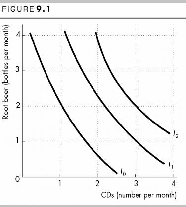
1. Marc has an income of $20 per week.

Root beer costs $5 a can and CDs cost

$10 each. Figure 9.1 illustrates his

preferences.

a. What are the quantities of root beer

and CDs that Marc buys?

b. What is Marc’s marginal rate of

substitution of CDs for root beer at the

point at which he consumes?

2. Now suppose that in the situation

described in problem 1, the price of a

CD falls to $5 and the price of root beer

and Marc’s income remain constant.

a. Find the new quantities of root beer

and CDs that Marc buys.

b. Find two points on Marc’s demand

curve for CDs.

c. Find the substitution e’ect of the price change.

d. Find the income e’ect of the price change.

e. Are CDs a normal good or an inferior good for Marc?

3. Pete buys tuna and golf balls. The price of tuna is $2 a can, and the price of a

golf ball is $1. Each month, Pete spends all of his income and buys 20 cans of

tuna and 40 golf balls. Next month, the price of tuna will rise to $3 a can and

the price of a golf ball will fall to 50¢. Assume that Pete’s preference map

shows indi’erence curves have a bowed in shape so that they show a

diminishing marginal rate of substitution.

a. Will Pete be able to buy 20 cans of tuna and 40 golf balls next month?

b. Will Pete want to buy 20 cans of tuna and 40 golf balls?

c. Which situation does Pete prefer: tuna at $2 a can and golf balls at $1 each

or tuna at $3 a can and golf balls at 50¢ each?

d. If Pete changes the quantities that he buys, which good will he buy more of

and which less of?

e. When the prices change next month, will there be an income e’ect and a

substitution e’ect at work or just one of them?

4. The sales tax is a tax on goods. Some people say that a consumption tax, a

tax on both goods and services, would be better. Explain and illustrate with a

graph what would happen if we replaced the sales tax with a consumption tax

a. The relative price of books and haircuts.

b. The budget line showing the quantities of books and haircuts you can a’ord

to buy.

c. Your purchases of books and haircuts.

1 0 0 C H A P T E R 9

S o l u t i o n s t o A d d i t i o n a l P r o b l e m s

1. a. Marc buys 2 cans of root beer and 1 CD. Marc buys the quantities of root beer and

CDs that moves him onto the highest indi’erence curve, given his income and the

prices of root beer and CDs. The graph shows Marc’s indi‘erence curves. So draw

Marc’s budget line on the graph. The budget line is tangential to indi’erence curve I0

at 2 cans of root beer and 1 CD. The indi’erence curve I0 is the highest indi’erence

curve that Marc can get attain.

b. Marc’s marginal rate of substitution is 2. The marginal rate of substitution is the

magnitude of the slope of the indi’erence curve at Marc’s consumption point, which

equals the magnitude of the slope of the budget line. The slope of Marc’s budget line

is 2, so the marginal rate of substitution is 2.

2. a. Marc buys 1 can of root beer and 3 CDs. Draw the new budget line on the graph with

Marc’s indi‘erence curves. The budget line now runs from 4 CDs on the x-axis to 4

cans of root beer on the y-axis. The new budget line is tangential to indi’erence

curve I1 at 1 can of root beer and 3 CDs. The indi’erence curve I1 is the highest

indi‘erence curve that Marc can now get attain.

b. Two points on Marc’s demand curve for CDs are the following: At $10 a CD, Marc

buys 1 CD. At $5 a CD, Marc buys 3 CDs.

c. The substitution e’ect is 1 CD. To divide the price e’ect into a substitution e’ect and

an income e’ect, take enough income away from Marc and gradually move his new

budget line back toward the origin until it just touches Marc’s indi’erence curve I0.

The point at which this budget line just touches indi’erence curve I0 is 2 CDs and 0.5

can of root beer. The substitution e’ect is the increase in the quantity of CDs from 1

CD to 2 CDs along the indi’erence curve I0. The substitution e’ect is 1 CD.

d. The income e’ect is 1 CD. The income e’ect is the change in the quantity of CDs

from the price e’ect minus the change from the substitution e’ect. The price e’ect

is 2 CDs (3 CDs minus the initial 1 CD). The substitution e’ect is an increase in the

quantity of CDs from 1 CD to 2 CDs. So the income e’ect is 1 CD.

e. CDs are a normal good for Marc because the income e’ect is positive.

3. a. Pete can still buy 20 cans of tuna and 40 golf balls. When Pete buys 20 cans of tuna

at $2 a can and 40 golf balls at $1 each, he spends $80 a month. Now that the price

of a can of tuna is $3 and the price of a golf ball is $0.50, 20 cans of tuna and 40

golf balls will cost $80. So Pete can still buy 20 cans of tuna and 40 golf balls.

b. Pete will not want to buy 20 cans of tuna and 40 golf balls because the marginal rate

of substitution does not equal the relative price of the goods. Pete will move to a

point on the highest indi’erence curve possible where the marginal rate of

substitution equals the relative price.

c. Pete prefers tuna at $3 a can and golf balls at $0.50 each because he can get onto a

higher indi’erence curve than when tuna is $2 a can and golf balls are $1 each.

d. Pete will buy more golf balls and fewer cans of tuna. The new budget line and the old

budget line pass through the point at 20 cans of tuna and 40 golf balls. If cans of

tuna are plotted on the x-axis, the marginal rate of substitution at this point on

Pete’s indi’erence curve is equal to the relative price of a can of tuna at the original

prices, which is 2. The new relative price of a can of tuna is $3/50 cents, which is 6.

That is, the budget line is steeper than the indi’erence curve at 20 cans of tuna and

40 golf balls. Pete will buy more golf balls and fewer cans of tuna.

e. There will be a substitution e’ect and an income e’ect. A substitution e’ect arises

when the relative price changes and the consumer moves along the same

P O S S I B I L I T I E S , P R E F E R E N C E S , A N D C H O I C E S 1 0 1

indi‘erence curve to a new point where the marginal rate of substitution equals the

new relative price. An income e’ect arises when the consumer moves from one

indi‘erence curve to another, keeping the relative price constant.

4. a. Books are goods and so are taxed under both a sales tax and a consumption tax.

Haircuts are services and so are taxed only under a consumption tax. If the sales tax

is replaced with a consumption tax, the relative price of a haircut rises and the

relative price of a book falls.

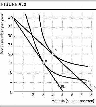
b. Assuming the sales tax and consumption

tax are the same rate, in the 0gure the

budget line rotates inward around a 0xed

book intercept. In Figure 9.2, the new

budget line is BL1. The price of a book

does not change but the price of a haircut

rises.

c. In general, if the relative price of a haircut

rises and the relative price of a book falls,

the substitution e’ect leads consumers to

buy more books and fewer haircuts. There

is, however, also an income e’ect. The

consumer’s real income falls, which

decreases the demand for normal goods.

Assuming that both books and haircuts

are normal goods, then the income e’ect

o’sets the substitution e’ect of buying

more books but reinforces the substitution

e’ect of buying fewer haircuts. In the 0gure, with the sales tax and budget line BL0

the consumer is initially at point A and buys 20 books per year and 4 haircuts per

year. With the consumption tax and budget line BL1 the consumer moves to point B

and buys 15 books per year and 3 haircuts per year.

A d d i t i o n a l D i s c u s s i o n Q u e s t i o n s

1. How does an increase in the price of basic food staples a ect real

income in poor countries? Illustrate this with a budget line and

hypothetical consumption bundle. Where money incomes are low,

increases in food prices can devastate real incomes and the achievable

consumption bundle. The budget line, already close to the origin, shifts inward

even closer. Food riots returned to the global stage in 2008, and with the prices

of many key grains rising in 2010, we may see continued global dialogue

about the negative impact of higher food prices on the world’s poorest citizens.

2. How would the preference map shift if a consumer had a strong

preference for one of the products versus the other? How might that

a ect the tangency point? The map tilts to be “long” on the axis of the

non-preferred product. Basically to get the person give up a unit of the

preferred product, compensation in terms of units of the other product to

maintain indi’erence would be immense. The tangency is thus likely to be

near the axis of the preferred product, which means a large quantity of this

good is consumed.

3. Will a low-income person’s optimal consumption bundle change if he

or she receives food stamps? Have the students apply a normal preference

mapping between food and all other goods for a low-income person. With food

1 0 2 C H A P T E R 9

on the vertical axis, show that a person receiving food stamps experiences a

new, steeper budget line with a higher y-intercept. Show that the person can

now a’ord a greater total amount of food for any given level of other goods,

but the maximum amount of all other goods available remains unchanged.

Have the students locate the consumption combination that matches the slope

of the new budget line with the marginal rate of substitution of the highest

indi‘erence curve.

Could the low-income person be better o with an income subsidy of

equal value to the food stamp subsidy? Show that if the same level of

income were given in place of food stamps, this opens up even more

combinations of goods and services than with food stamps. It is impossible not

0nd a higher indi’erence curve without a very unconventional indi’erence

curve map.

Could a low-income person be made equally as well o with a lower

total income subsidy than the initial food stamp subsidy? Ask them to

consider why the government continues to use food stamps instead of income

assistance when the same quantity of extra income would bring them even

more utility. Ask them why the government doesn’t minimize total welfare

assistance expenditures by giving them just enough income to maintain a

consumption bundle on the same indi’erence curve as with the current food

stamp expenditures. Students should recognize that part of the government’s

intention is to control the type of items purchased with food stamps. If

low-income households were simply given cash subsidies, the costs of the

welfare system would be lower, but not all low-income households would

spend that cash subsidy on food only.

4. Would the indi erence curves of a preference map ever change shape

when the prices of goods change? Marketing managers for Ferrari claim

that they would not consider a signi0cant price decrease in the face of falling

demand. They worry that the decrease in the perceived “exclusivity” of the

brand would diminish the consumer perception of their product and eventually

decrease market demand. Ask the students to model this theory and show how

a sharp decline in the price of a Ferrari might causes a change in the

consumer’s indi’erence curves. (The answer is that if Ferraris were placed on

the vertical axis, the indi‘erence curves are steeper.)

Would indi erence curves ever move whenever the consumer’s

income changes? Consumers change their buying habits as they increase

their income. They buy cars with leather seats instead of cloth, designer

dresses and purses, choose restaurants merely to “be seen” dining there. Does

this really represent a change in the preference mapping over consumption

possibilities when incomes increase? Does it change the slope of the

indi‘erence curve?

5. Do perfect substitutes imply perfectly elastic demand? When

indi‘erence curves are straight lines, the MRS is almost never equal to the

relative price ratio, meaning the consumer selects a “corner solution” (all of

one good, or all of another, but not a mix of both). In the case of a relative

price change, the consumer immediately switches to consuming only the other

good. Ask the students if they have ever observed such peculiar consumer

behavior in the real world.

Do perfect complements imply perfectly inelastic demand? When the

indi‘erence curves are 90-degree angles, the consumer always purchases the

product only in exact proportions. Ask the students if there is any usefulness to

separating out the two goods as separate items, or whether it is more

P O S S I B I L I T I E S , P R E F E R E N C E S , A N D C H O I C E S 1 0 3

meaningful to consider them two necessary components of a single good. For

example, we rarely see single shoes being o’ered for sale, but surely the

occasional consumer loses a single shoe, or there are a small number of

amputees that need only one shoe. Why is there no market for single shoes?

(As a counterexample, Lands’ End actually sells single gloves or mittens to

consumers who have lost one of a pair.)

1 0 4 C H A P T E R 9