
T h e B i g P i c t u r e
Where we have been:
This chapter develops a more thorough understanding of eciency, which was
rst introduced in Chapter 2. It also develops a deeper grasp of how the
demand and supply model introduced in Chapter 3 inuences resource
allocations in an economy. Finally, it explains the situations in which a
competitive market does and does not allocate resources eciently.
Where we are going:
Chapter 6 applies the concepts of eciency and deadweight loss to market
regulation policies such as rent ceilings and minimum wage laws. Students
should understand these concepts well to appreciate applying demand and
supply to important markets in our economic world. Chapter 7 then applies the
same concepts to issues surrounding international trade and government
protectionist policies. The concepts of eciency and deadweight loss recur in
Chapters 12, 13, and 14, which examine perfect competition, monopoly,
monopolistic competition, and regulation. The same eciency concepts are
also used in Chapters 16 and 17, which cover social issues such as public
goods and externalities.
N e w i n t h e Tw e l f t h E d i t i o n
The chapter opener examines trac and driving choices, which is then more deeply
analyzed in the Economics in the News section at the end of the chapter. The
Economics in Action: Selling the Invisible Hand application has been update with a
new real-world example on pizza delivery. A new Worked Problem section has been
added. The Worked Problem presents a supply and demand diagram and then shows
the students how to illustrate the consumer surplus and producer surplus. It also
shows the students how to determine if a market is ecient and how to calculate the
deadweight loss if an inecient quantity is produced. To include the new Worked
Problem without lengthening the chapter, some problems have been removed from
the Study Plan Problem and Applications. These problems are in the MyEconLab and
are called Extra Problems.e Notes
C h a p t e r

Eciency and Equity
Using prices in markets to allocate scarce resources is one of many alternative
methods of allocating scarce resources.
Tools such as consumer surplus and producer surplus help evaluate eciency.
The outcomes from the various methods used to allocate scarce resources,
especially markets, can be examined in terms of both their eciency and fairness.
I. Resource Allocation Methods
Resources are scarce, so they somehow must be allocated. Di9erent methods of allocating
resources include:
Market price: The people who are willing and able to buy a resource get the resource.
Command: a command system allocates resources by the order (command) of
someone in authority. A command system works well in organizations with clear
lines of authority but does not work well at allocating resources in the entire
economy.
Majority rule: resources are allocated in accordance with majority vote. Majority rule
works well when the allocation decisions being made a9ect a large number of people
and self-interest leads to bad decisions.
Contest: resources are allocated to the winner. Contests work well when the e9orts of
the players are hard to measure, such as top managers being in a contest to be
named CEO of a company.
First-come, rst-serve: resources are allocated to those who are rst in line. This
allocation method works well when the resource can serve just one user at a time in
a sequence, as is the case with, say, a bank teller or an ATM.
Lottery: resources are allocated to the people who pick the winning number, choose
the lucky card, etc. Lotteries work best when there is no e9ective way to distinguish
among potential users of a scarce resource.
Personal characteristics: resources are allocated to people with the “right”
characteristics.
Force: resources are allocated to those who can forcibly take the resources.
Is allocating goods to those willing and able to pay higher prices fundamentally
unfair? Students often believe that allocating resources using market prices is somehow
unfair. The rst section of this chapter, which discusses di9erent ways of allocating
resources, and the discussion in the last section of the chapter about the fairness of these
di9erent methods in a situation with a shortage, will help open students’ eyes to the fact
that somehow resources must be allocated and using the market price has many desirable
characteristics that are perhaps often overlooked. In particular, using market prices to
allocate goods and services means that goods and services are sold to people who can
a9ord them and want to buy them. Students often focus on the rst part—“a9ord”—and
ignore the second part—“want to buy.” Clearly wealthy people can better a9ord to buy
goods and services. But this does not mean that the wealthy buy everything. For instance,
it is likely the case that your cell phone is less advanced in features and service plans than
cell phones owned by your students. You perhaps can better a9ord these phones than your
students, but you simply may not want the newest, most wired smart device as much as
they do. So using market prices means that people who most strongly want the newest and
greatest smart phone will acquire it … at least as long as they can a9ord it. Other resource
allocation methods generally do not take account of how strongly someone wants a good
or service. As a result, other methods of allocation can allocate goods and services to
people who may not value them the most.
II. Benet, Cost, and Surplus
Demand, Willingness to Pay, and Value
The value of one more unit of a good or service is its marginal benet. Marginal
benet is the maximum price that people are willing to pay for another unit of a
good or service. And the willingness to pay for a good or service determines the
demand for it. Consequently the demand curve for a good or service is also its
marginal benet curve.
The market demand curve is the horizontal sum of the individual demand curves
and is formed by adding the quantities demanded by all the individuals at each
price.
How do you add “horizontally”? Students sometimes have trouble with the concept of
adding individual demand curves “horizontally.” Emphasize that the quantity demanded is
measured on the “horizontal” axis, so we’re simply adding together all the individual
quantities demanded to get the market quantity demanded at a particular price.
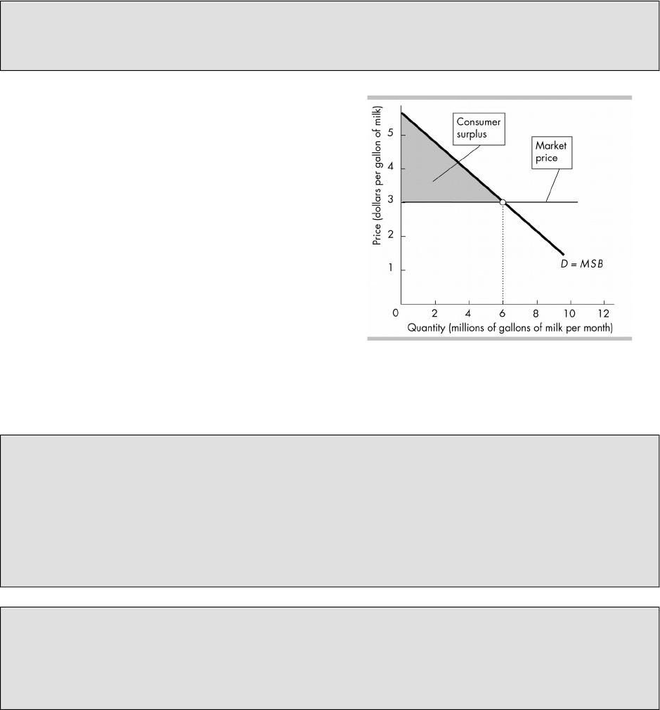
The demand curve in the gure shows
that the maximum price a person is
willing to pay for the 6 millionth gallon of
milk per month is $3, so $3 is the
marginal benet of this gallon.
MSB curve: In the absence of
externalities, which will be discussed
later, the market demand curve is also
the economy’s marginal social benet
(MSB) curve. It reects the number of
dollars’ worth of other goods and
services willingly given up to obtain one
more unit of a good.
The gure shows that the maximum
price a consumer is willing and able to
pay for the 6 millionth gallon of milk is
$3, so the marginal social benet of the 6 millionth gallon of milk is $3.
Consumer surplus is the value (or marginal benet) of the good minus the price
paid for it, summed over the quantity bought. The gure illustrates the consumer
surplus as the shaded triangle when the price is $3 per gallon.
The negative slope of demand and declining marginal bene#t. Marginal benet is
the maximum price people are willing to pay for one more unit of a good or service.
Because willingness to pay determines demand, a demand curve is a marginal benet
curve. Demand curves have a negative slope because, as the price rises, the quantity
demanded falls. The negative slope of the demand curve can also be explained by the
concept of declining marginal benet. The more you already have of a good, the less
valuable an additional unit of that good is to you. In other words, the maximum price you
are willing to pay for another unit of that good (its marginal benet) declines as the
quantity you have increases.
Consumer surplus graphically is the area under the demand curve and above the
price. One thing that students sometimes get hung up on is the exact shape of the
consumer surplus area, in particular the steps of consumer surplus for discrete units
versus the complete triangle. The point isn’t worth laboring, but if students raise the
matter and are curious, you might explain that we’re assuming that the good is nely
divisible so that the whole triangle is (approximately) the consumer surplus.
Low prices are great for consumers. Students know that low prices are better for
consumers than high prices. But consumer surplus gives them a way to demonstrate this
basic idea. Take a minute to evaluate the change in consumer surplus from a given change
in price. The big impact is not the marginal increase in the number of units purchased, but
the increase or decrease in consumer surplus of the units that are still being purchased
regardless of the change in price. The area of consumer surplus will become smaller when
prices rise and larger when prices fall. This quanties graphically something students
intrinsically know: from the point of view of consumers, low prices are good and high prices
are bad. The best example for most people is their strong irritation when gas prices rise
and their perception of well being when gas prices fall. Even if they do not change the
amount of gas they buy at all, they perceive the change in their consumer surplus.
Supply, Cost, and Minimum Supply-Price
The cost of producing one more unit of a good or service is its marginal cost.
Marginal cost is the minimum price that producers must receive to induce them to
produce another unit of the good or service. And the minimum acceptable price
determines the quantity supplied. Consequently the supply curve for a good or
service is also its marginal cost curve.
The positive slope of supply and increasing marginal cost. The fact that supply
curves have a positive slope implies that the marginal cost of production increases as the
level of production expands. You can refer back to increasing opportunity costs to reinforce
this idea for your students. As producers increase production, they will need to increase the
amount of resources they use. Initially, rms use the cheapest resources possible (labor
that has comparative advantage in producing the good, for example). As output expands,
however, additional resources will become increasingly costly (as labor that does not have
a comparative advantage in production is used in the production process). If resource costs
are rising as the quantity of output supplied increases, the minimum price producers must
receive to induce them to produce more will also increase.
The market supply curve is the horizontal
sum of the individual supply curves and is
formed by adding the quantities supplied by
all the producers at each price.
MSC curve: In the absence of externalities,
the market supply curve is the economy’s
marginal social cost (MSC) curve.
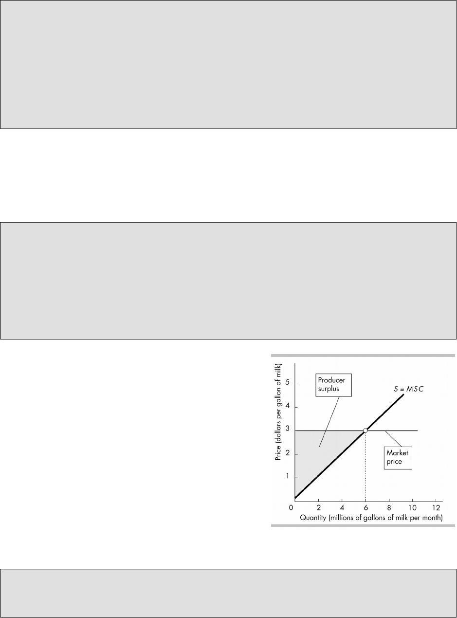
The supply curve in the gure shows that
the minimum price a producer must
receive to be willing to produce the 6
millionth gallon of milk per month is $3,
so $3 is the marginal social cost of this
gallon.
Producer surplus is the price of a good
minus its minimum supply-price (or
marginal cost), summed over the quantity
sold. The gure illustrates the producer surplus as the shaded triangle when the
price is $3 per gallon.
Producer surplus graphically is the area above the supply curve and below the
price line. Every unit that adds more to revenue than it does to cost adds to producer
surplus. Point out how increases in price expand producer surplus and how decreases in
price reduce it. From producers’ point of view, high prices are better, something that often

confuses students who are used to thinking of price as cost not as revenue. This is a good
moment to reinforce that di9erence.
Is producer surplus the same as pro#t? At this point in the course, students don’t have
all the tools necessary to understand the di9erence so it is perhaps best to simply say they
aren’t exactly the same, and that rms will sometimes nd it in their best interests to
produce for a time even if they are losing money. Promise to explore prot and
prot-maximization more in future chapters. If students are persistent you can explain that
producer surplus equals total revenue minus total variable cost, while economic prot
equals total revenue minus total cost. That means producer surplus isn’t exactly economic
prot. Rather, producer surplus equals economic prot plus total xed cost. Don’t spend
much time discussing this point now, but be ready for it if you get such a question when
you’re in Chapters 12, 13, or 14.
III. Is the Competitive Market E%cient?
Eciency of Competitive Equilibrium
The marginal benet to the entire society is
the marginal social benet curve, MSB. If all
the benets from consuming a good go to its
consumers, the market demand curve is the
same as the MSB curve.
The marginal cost to the entire society is the
marginal social cost curve, MSC. If all the
costs of producing a good are paid by the
producers, the market supply curve is the
same as the MSC curve.
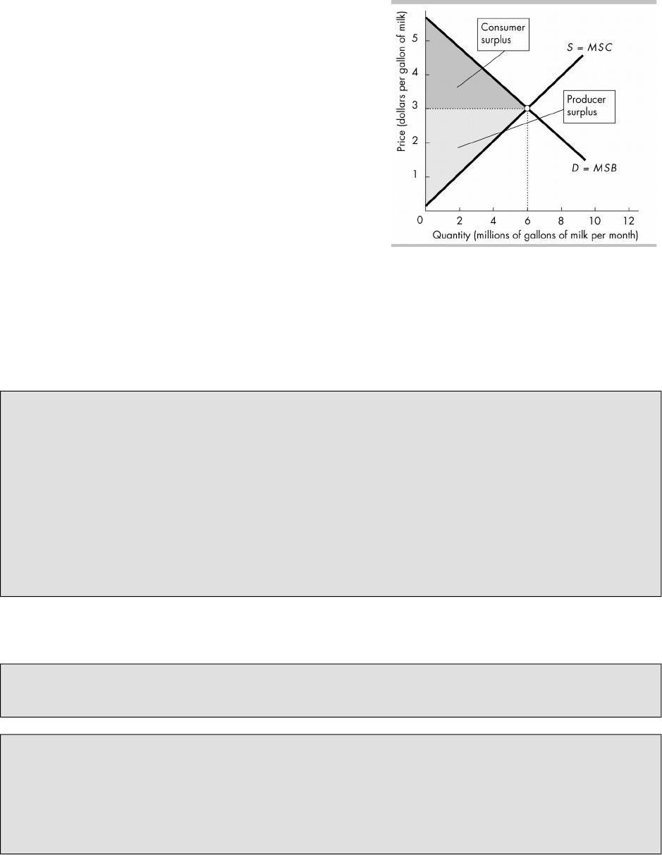
When the marginal social benet of the last
unit produced equals its marginal social
cost, society attains eciency. However,
because the demand curve is the same as the MSB curve and the supply curve is the
same as the MSC curve, the ecient quantity that sets the MSB equal to the MSC
also sets the quantity demanded equal to the quantity supplied and so is the
equilibrium quantity. The gure illustrates how the ecient quantity of milk, 6
million gallons per month, also is the equilibrium quantity of milk.
When the ecient quantity of milk is produced, the sum of the consumer surplus
and producer surplus (total surplus) is maximized.
It helps to summarize all the results of eciency at this point, as follows:
By denition, eciency requires that resources are being used where they are most
highly valued.
When resources are used where they are most highly valued, MSB = MSC.
When the demand and supply curves intersect, QD = QS, and the market achieves
equilibrium.
At equilibrium the total surplus in the market is maximized. (This is usually the most
dicult concept to prove without use of calculus in principles courses. Be sure to
emphasize to your students that the following sections and chapters will show exactly
what happens to consumer and producer surplus when the market moves away from
equilibrium.)
Buyers and sellers acting in their own self-interest maximize social well-being.
Adam Smith, in his 1776 book The Wealth of Nations, articulated how competition
led self-interested consumers and producers to make choices that unintentionally
promote the social interest as if they were led by an “invisible hand.
Economics in Action: Selling the Invisible Hand
This case discusses how the Invisible hand of the market allocates resources to their
highest valued use rst with a cartoon and then in a real-life case of pizza delivery.
The Invisible Hand at work: When demand or supply shifts in a market, equilibrium
changes to a new point where the MSB = MSC, as reected in the new demand or supply
curve. Show students how an increase in demand, for example, increases the MSB of every
unit of output and results in a new, higher level of output that achieves eciency. A
decrease in supply raises the MSC of every unit, and with fewer units available, the MSB of
those units is greater. The resulting decrease in output from the change in supply achieves
eciency.
For students who want more information: Although done simply with words and a
graph, this section explains the so-called “rst fundamental theorem of welfare
economics” that, under appropriate conditions, the competitive equilibrium is Pareto
ecient (what this textbook calls an “ecient allocation”). You can extend Adam Smith’s
“invisible hand” conjecture with mention of Vilfredo Pareto (1848–1923), an Italian
economist who dened an ecient allocation as one in which it is not possible to rearrange
the use of resources and make someone better o9 without making someone else worse o9.
But Adam Smith’s conjecture did not receive formal proof until the 1950s. John Hicks,
Kenneth Arrow, and Gerard Debreu are credited with the major contributions to welfare
economics and received the Nobel Prize in Economic Sciences.
(http://www.nobel.se/economics/laureates/1972/index.html,
http://www.nobel.se/economics/laureates/1983/index.html). Lionel McKenzie (University of
Rochester) is also credited with a major independent statement of the theorem and some
economists refer to it as the Arrow-Debreu-McKenzie theorem. The A-D-M proof is deeper
and more restricted than the words and diagrams of a principles text. But we do not
mislead our students by being enthusiastic and amazed at the astonishing proposition.
Selsh people all pursuing their own ends and making themselves as well o9 as possible
end up allocating resources in such a way that no one can be made better o9 (qualied by
the exceptions that we quickly note in the chapter.)
Market Failure
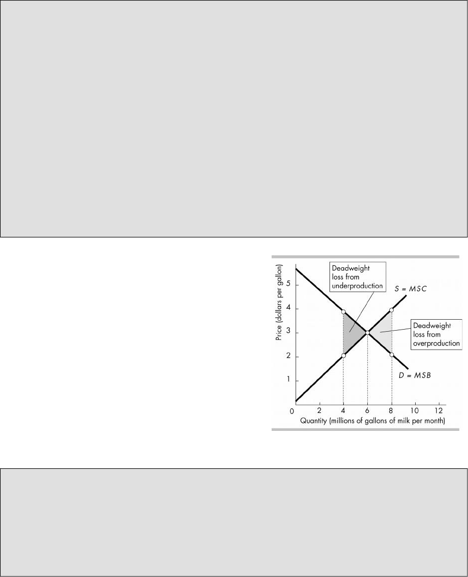
Ineciency can occur because either too
little of an item is produced
(underproduction) or too much is produced
(overproduction).
In either case, a deadweight loss occurs. A
deadweight loss is the decrease in the
consumer surplus and producer surplus
(decrease in total surplus) that results from
producing at an inecient level of
production. The gure illustrates the
deadweight loss from overproduction of
milk and from underproduction
What is deadweight loss intuitively? In the gure above, production of the 4 millionth
gallon of milk results in a MSB of $4 and a MSC of $2. By stopping production at 4 million
gallons, society is losing that extra $2 of benet relative to cost. In fact, the MSB will be
greater than MSC for all production less than 6 million gallons. That lost value to society is
deadweight loss. Similarly, production of the 8 millionth gallon of milk results in a MSB of
$2 and a MSC of $4. In this case, the resources used to produce any milk beyond the 6
millionth gallon impose an additional cost that is greater than its additional benet. In
other words, resources would have a higher value elsewhere (in their best alternative use)
than their use in the production of milk. That lost value to society again is deadweight loss.
Sources of Market Failure
Sometimes a market overproduces or underproduces a good or service. The key obstacles
to achieving an ecient allocation of resources in a market are:
Price and Quantity Regulations: A price ceiling sets the highest legal price and a
price oor sets the lowest legal price. If a price ceiling or price oor makes the
equilibrium price illegal, it can lead to ineciency. Quantity regulations that limit the
amount produced also lead to ineciency. (Studied in Chapter 6)
Taxes and Subsidies: Taxes and subsidies place a wedge between the prices
consumers pay and the prices producers receive. Both can lead to ineciency.
(Studied in Chapter 6)
Externalities: An externality is a cost or a benet that a9ects someone other than
the seller or the buyer. In that case, the demand curve is not the same as the
marginal social benet curve and/or the supply curve is not the same as the
marginal social cost curve. In these cases, ineciency results. (Studied in Chapter
16)
Public Goods and Common Resources: A public good is a good or service that is
consumed simultaneously by everyone even if they don’t pay for it. Public goods
lead to a free-rider problem, in which people do not pay for their share of the good. A
common resource is owned by no one but available to be used by everyone.
Common resources are generally over-used because no one owns the resource. In
both cases, ineciency can occur. (Studied in Chapter 17)
Monopoly: A monopoly is a rm that has sole control of a market. To maximize its
prot, a monopoly produces less than the ecient quantity and so creates
ineciency. (Studied in Chapter 13)
High transactions costs: The opportunity costs of making a trade are transactions
costs. When these costs are high, a market might underproduce because too few
transactions take place.
Alternatives to the Market
If markets do not allocate resources eciently, then one of the alternatives might do a
better job. For instance, using rst-come, rst-serve to allocate spaces in a line at a movie
theater probably works better than a market.