
T h e B i g P i c t u r e
Where we have been:
The student can now use the demand and supply model to generate
predictions and can supplement this knowledge with the ability to provide
richer predictions based on the elasticities of demand and supply.
Where we are going:
Demand, supply, and demand elasticity get an extensive workout in Chapter 6,
where we use them to explain the division of a tax burden between buyer and
seller and the impact of price controls and quotas. However, before doing that
analysis, we study the e!ciency and fairness of markets in Chapter 5.
Students will also apply elasticity in Chapter 12 to describe demand in perfect
competition. In Chapter 13, we study the relationship between total revenue
and the price elasticity of demand to show that a monopoly never operates on
the inelastic part of the demand curve.
N e w i n t h e Tw e l f t h E d i t i o n
There are only a few minor changes to this chapter. A new introduction and
application focus on the co)ee market and the elasticity of demand for co)ee. Two
new Economics in the News applications examine demand elasticities for peanut
butter in the United States market. A New Worked Problem is included. The Worked
Problem presents data on changes in the price and quantity of smoothies and
changes in the quantity of mu!ns. It asks the students to calculate the
percentage changes in the price and quantity of smoothies, the price elasticity of
demand for smoothies, and the cross elasticity of demand for mu!ns with respect
to the price of a smoothie. The Worked Problem then shows the students how to
make these calculations. To include the new Worked Problem without lengthening
the chapter, some problems have been removed from the Study Plan Problem and
Applications. These problems are in the MyEconLab and are called Extra Problems.
© 2016 Pearson Education, Inc.
C h a p t e r
37
3 7

L e c t u r e N o t e s
Elasticity
The price elasticity of demand measures how strongly buyers respond to a change in
the price of a good.
The price elasticity of demand can be used to make quantitative predictions of how
changes a)ect the price and quantity demanded of a good.
The income elasticity of demand measures how strongly demanders respond to a
change in income, and the cross elasticity of demand measures how strongly
demanders respond to the change in the price of another good.
The price elasticity of supply measures how strongly producers respond to a change
in the price of a good.
I. Price Elasticity of Demand
In general, elasticity measures responsiveness. The price elasticity of demand
measures how responsive demanders are to a change in the price of the good. This
information is often useful for both businesses and governments because it can
predict the impact of a price change on total revenue or total expenditure.
Calculating Price Elasticity of Demand
The price elasticity of demand is a units-free measure of the responsiveness of
the quantity demanded of a good to a change in its price when all other in5uences
on a buyer’s plans remain unchanged. The price elasticity of demand is equal to the
absolute value of:
Percentage change in quantity demanded
Percentage change in price .
The formulas for calculating all of the elasticities in the text are based on the arc elasticity
or mid-point formula, meaning the percentage changes are always calculated based on
the average price (or income in the case of income elasticity) and average quantity over
the range of change. If you ask students to calculate elasticities, it is important to practice
calculating the percentage change using the average as the basis as it is not likely to be
familiar Don’t be afraid to start with this pre-elasticity warm up to assess the sharpness of
your class. Ask: “Suppose that the campus bookstore increases the price of an economics
text from $75 to $100. What is the percentage increase in price?” Many will say 25 percent.
But using the midpoint formula the percentage change is ($25/$87.50) × 100, which is
28.6 percent.
Devise a mnemonic for elasticity calculations. Many students have a hard time
remembering whether quantity or price goes in the numerator of the elasticity formulas.
Have the students create their own mnemonic. Suggest McDonald’s Quarter Pounder™
hamburgers. It’s silly, but it works, reminding the student that Q (quantity) appears before
P (price) in the ratio of percentage changes.
The demand elasticity formula yields a negative value, because price and quantity
move in opposite directions. However, it is the magnitude, or absolute value, of the
measure that reveals how responsive the quantity change has been to a price
change. So we use the magnitude or the absolute value of the price elasticity of
demand.
The table to the right has two points on the
demand curve for pizza from a particular
pizza parlor.
Price
(dollars per
pizza)
Quantity
demanded
(pizzas per
week)
14 500
16 400
The absolute value of the percent change in quantity demanded is
[(500 400) 450] 100 = 22.2 percent.
The absolute value of the percentage change in price is
[($14 $16) $15] 100 = 13.3 percent.
Between these two points on the demand curve, the price elasticity of demand is
22.2% 13.3% = 1.67.
Elasticity is not the same as slope. Students sometimes wonder why we don’t just
measure the slope of the demand curve to measure responsiveness. Point out to the
students that the slope will change when the units change. For instance, you can compute
the slope of a demand curve when the price is measured in dollars and then the slope of
the exact same demand curve when the price is measured in cents. The slope with the
price measured in cents is 100 times as large as the initial slope. Tell the students that it is
not acceptable for the measure of responsiveness to change whenever the units of the
price (or of the quantity) change.
Inelastic and Elastic Demand
If the price elasticity of demand is less than 1.0, the good is said to have an
inelastic demand. In this case, the percentage change in the quantity demanded is
less than the percentage change in price.
If the quantity demanded remains constant when the price changes, then the
good is said to have perfectly inelastic demand. The price elasticity of
demand is 0 and the good’s demand curve is a vertical line.
If the price elasticity of demand is equal to 1.0, the good is said to have a unit
elastic demand. In this case, the percentage change in the quantity demanded
equals the percentage change in price.
If the price elasticity of demand is greater than 1.0, the good is said to have an
elastic demand. In this case, the percentage change in the quantity demanded
exceeds the percentage change in price.
If the quantity demanded changes by an
inMnitely large percentage in response to a
tiny price change, then the good is said to
have perfectly elastic demand. The price
elasticity of demand is inMnite.
The table has some “real-life” elasticities from the
book.
Economics in Action” Elastic and Inelastic Demand
This application shows real-world price elasticities of demand for a variety of goods and
services as well as a table with various food elasticities. This data can be a base for
discussion of the factors that might lead one item to be more elastic than the other and
allow students in real-time to try to explain and apply price elasticity of demand.
Economics in the News: The Elasticity of Demand for Peanut Butter
The price elasticity of demand for peanut butter
is the basis for this application. Further
discussion of other demand elasticities for
peanut butter will be explored after those
elasticities are introduced.
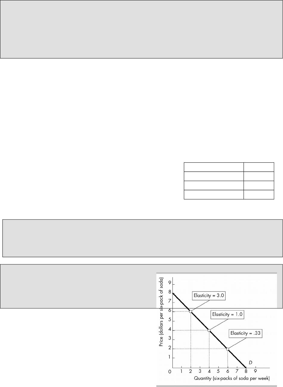
Elasticity Along a Linear Demand Curve
With the exception of a vertical demand
curve and a horizontal demand curve
(along which the elasticity is 0 and
Furniture 1.26
Motor Vehicles 1.14
Clothing 0.64
Oil 0.05

inMnite, respectively) the price elasticity of demand changes when moving along a linear
demand curve.
As the Mgure illustrates, at points on the demand curve above the midpoint, the
price elasticity of demand is elastic while at points below the midpoint, the price
elasticity of demand is inelastic. At the midpoint, the price elasticity of demand is unit
elastic.
Total Revenue and Elasticity
The total revenue from the sale of a good equals the price of the good multiplied
by the quantity sold.
If demand is elastic, a 1 percent price cut increases the quantity sold by more
than 1 percent and total revenue increases.
If demand is unit elastic, a 1 percent price cut increases the quantity sold by 1
percent and total revenue does not change.
If demand is inelastic, a 1 percent price cut increases the quantity sold by less
than 1 percent and total revenue decreases.
The total revenue test is a method of estimating the price elasticity of demand by
observing the change in total revenue that results from a change in price, when all
other in5uences on the quantity sold remain the same.
If a price cut increases total revenue, demand is elastic. And if a price hike
decreases total revenue, demand is elastic.
If a price cut does not change total revenue, demand is unit elastic. And if a price
hike does not change total revenue, demand is unit elastic.
If a price cut decreases total revenue, demand is inelastic. And if a price hike
increases total revenue, demand is inelastic.
Similarly, when a price changes, a consumer’s change in expenditure depends on
the consumer’s elasticity of demand.
If demand is elastic, then a price cut means that expenditure on the item
increases.
If demand is inelastic, then a price cut means that expenditure on the item
decreases.
If demand is unit elastic, then a price cut means that expenditure on the item
does not change.
How do changes in revenue relate to elasticity mathematically? When demand is
elastic, the absolute value of the ratio of the percentage change in quantity demanded to
percentage change in price must be greater than one. This point implies that the
numerator of the formula for the price elasticity of demand must be greater than the
denominator. In that case, the percentage change in quantity demanded is stronger than
the percentage change in price, so revenues will change in the same direction as the
quantity demanded. On the other hand, if demand is inelastic, the denominator of the
formula for the price elasticity of demand must be greater than the numerator. In that
case, changes in revenue will change in the same direction as the price because the
percentage change in price is stronger than the percentage change in quantity. Reviewing
these results also helps students understand the logic for why 1 is the signiMcant value for
the coe!cient and that the elasticity being farther away from 1 means the reaction is
stronger, whether elastic or inelastic.
The Factors that In uence the Elasticity of Demand
The magnitude of the price elasticity of demand depends on:
The closeness of substitutes: The closer and more numerous the substitutes for a
good or service, the more elastic the demand. This is critical for understanding
demand in the market structure section later in the book.
The proportion of income spent on the good: The greater the proportion of income
spent on a good or service, the more elastic the demand.

The amount of time elapsed since the price change: The longer the time elapsed
since the price change, the more elastic the demand.
Price elasticity of needs versus wants: Necessities, such as food or housing, generally
have inelastic demand because there are few substitutes for food and shelter. Luxuries,
such as exotic vacations, generally have elastic demand. Example: Most people’s demand
for salt is inelastic, largely because most people spend a miniscule amount of their income
on salt. However large Northern cities’ demand for salt is signiMcantly more elastic. These
cities use salt to treat their roads after a snow storm. Salt is a signiMcant fraction of their
budgets. Because the proportion of their income they spend on salt is large, the price
elasticity of demand for these cities is much larger than that of “ordinary” consumers.
How do gasoline purchases respond to changes in price over time? When gas
prices rise from $2 to $4, consumers initially have few options available. At Mrst, with a
given car with a given gas mileage, higher gas prices do not reduce the quantity of gas
consumers purchase by very much. As time passes and gasoline prices continue to remain
high, some consumers eventually Mnd ways to adjust their gas purchases by purchasing
more fuel e!cient cars, taking new jobs that are closer to their homes, or by taking fewer
road trips or car pooling.
II. More Elasticities of Demand
Income Elasticity of Demand
The income elasticity of demand is a measure of the responsiveness of the
demand for a good to a change in the income, other things remaining the same.
The income elasticity of demand is equal to:
Percentage change in quantity demanded
Percentage change in income .
The changes in the quantity demanded and income are percentages of the average
income and quantity demanded over the range of change.
The income elasticity of demand is positive for normal goods and negative for
inferior goods.
If the income elasticity of demand is greater than 1, demand is income elastic
and the good is a normal good. As income increases, the percentage of income
spent on income elastic goods increases.
If the income elasticity of demand is positive but less than 1, demand is income
inelastic and the good is a normal good. As income increases, the percentage of
income spent on income inelastic goods
decreases.
If the income elasticity of demand is negative the
good is an inferior good.
The table has some “real-life” income elasticities
from the book.
One of the more common applications for income elasticity of demand that student’s tend
to Mnd interesting is in the stock market. Terms like cyclical, staples, and discretionary
sectors are easily explained using income elasticity concepts. Students could consider
questions about where in the business cycle a company’s proMt might be strongest or
weakest and thus more or less worthy of Mnancial investment.
Economies in Action: The Economics in Action shows actual estimates of income and
cross price elasticities. Grocery stores and retail stores are a great example of how store
Airline Travel 5.82
Restaurant Meals 1.61
Clothing 0.51
Food 0.14

scanned data could be used to understand the relationships between products. If a store
can put a low margin product on sale and sell more of a high margin product, that is a
great use of cross price elasticity data.
Cross Elasticity of Demand
The cross elasticity of demand is a measure of the responsiveness of the
demand for a good to a change in the price of a substitute or complement, other
things remaining the same.
The cross elasticity of demand is equal to:
Percentage change in quantity demanded
Percentage change in price of a substitute or complement .
The changes in the quantity demanded and the price are percentages of the
average price and quantity demanded over the range of change.
The cross elasticity of demand is positive for substitutes and negative for
complements.
Examples: Use examples to show the students why the cross elasticity of demand is
positive for substitutes and negative for complements. For instance, suppose the price of
Coke rises. What e)ect does this price hike have on the demand for Pepsi? Students will
immediately realize that the demand for Pepsi increases. So in this case the cross elasticity
of demand for Pepsi with respect to the price of Coke is calculated by dividing one positive
number by another, so the result will be positive. (You may need to show the result of a
decrease in the price of Cock as well: If the price of Coke falls, the demand for Pepsi will
fall, and the cross elasticity of demand for Pepsi with respect to Coke is calculated by
dividing a negative percentage change by a negative percentage change, again resulting
in a positive number.) Use speciMc percentage changes to calculate cross price elasticities
to emphasize that the sign of the coe!cient matters as well as its size. A cross elasticity of
1.5 or .3 are both substitutes but not to the same degree. A cross elasticity of 0.6 or 2.5
are both complements, but again not equally impactful. Explore how knowing cross
elasticities might help store managers plan “loss leaders” or how to merchandise products
each week.
Some instructors will be more focused on the calculation of the elasticities while others
may be more focused on interpreting the elasticity coe!cients. For those focused on
interpretation, tables with elasticity coe!cients could be provided and questions could be
framed in terms of the business cycle and how it would change sales of various products at
various stores. One store that caters to higher income customers and one store that has
bargain basement prices will have di)erent amounts of shelf space devoted to di)erent
products. More data would be needed for calculating the elasticities, but students could
then create the table and answer the interpretive questions as an class or take home
application.