
W H AT I S E C O N O M I C S ? 2 3
T h e B i g P i c t u r e
Where we have been:
In Chapter 3, the students have their rst encounter with demand and supply
and the powerful forces that determine price and quantity in a competitive
market. Chapter 3 builds on Chapter 2, which provides the simplest rigorous
description of the economic problem and the implications of the pursuit of an
e*cient use of resources. If you have time, it is worth forging links between
Chapters 2 and 3. Chapter 2 explains why we trade in markets. Chapter 3
shows how trade in markets determines where on the PPF the economy
operates.
Where we are going:
Demand and supply lie at the heart of the principles course. Eventually in the
microeconomics class we derive the demand curve and the supply curve from
deeper views of the choices that people and rms make. And in the
macroeconomic class, the lessons learned here apply, albeit with subtle
di-erences, to the aggregate supply-aggregate demand model.
N e w i n t h e T w e l f t h E d i t i o n
The content of this chapter is largely the same except for the Economics in the
News sections, which are now replaced with new current topics of co-ee and
bananas. The banana article is at the end of the chapter along with the extended
Economic Analysis of the end-of-chapter articles. There is a reduction in the
section covering all possible shifts of demand and supply. The content now focuses
on situations where both curves shift, which allows for two simpler gures to be
used to illustrate shifts. The single shifts of curves are already covered earlier so
there is no loss of content. There is a new Worked Problem at the end of the
chapter. The Worked Problem gives demand and supply schedules for roses and
then asks the students how the market adjusts if the price is lower and higher
than the equilibrium price. It follows up by asking the students to determine the
equilibrium price and quantity. Then the Worked Problem asks the students to
calculate new equilibrium prices and quantities when the supply changes and
when the demand and supply both change. The Worked Problem shows the
students how to make these calculations. In particular, it demonstrates how to
calculate the new equilibrium when the demand and supply change using the new
demand and supply schedules and using a supply and demand diagram. To
3DEMAND AND
SUPPLY
C h a p t e r
23
2 4
include the new Worked Problem without lengthening the chapter, some problems
have been removed from the Study Plan Problem and Applications. These
problems are in the MyEconLab and are called Extra Problems.
24
L e c t u r e N o t e s
Demand and Supply
In our market-based economy, the interaction of demand and supply in markets
determines the prices of goods and services and the quantity produced and
consumed.
Changes in demand and/or supply lead to changes in the price of the good or service
and in the quantity produced and consumed.
Markets vary in the intensity of competition. This chapter studies a competitive
market, which is a market that has many buyers and sellers, so no single buyer or
seller can in4uence price.
The money price of a good or service is the number of dollars that must be given
up for it. The ratio of one (money) price to another is called a relative price. A
relative price is an opportunity cost. The theory of demand and supply determines
relative prices and so when we use the word “price” we mean “relative price.”
To point out the importance of relative prices, ask your students if turkey at 40¢ a pound is
a good buy. Tell them that is all they know—turkey is 40¢ a pound. Generally most students
respond that turkey at this price is cheap and a good buy. Then tell them that steak is 8¢ a
pound. Now is turkey such a good buy? Students realize that the relative price of turkey is
5 pounds of steak per pound of turkey and so turkey is actually expensive. Point out to
them that these money prices are actual prices from circa 1800. At that time, turkey was
relatively quite expensive because turkeys could 4y and needed to be hunted rather than
harvested! Also point out to them the unimportance of the money price and the crucial
importance of the relative price.
I. Demand
The price of a good or service a-ects the quantity people plan to buy. The quantity
demanded of a good or service is the amount that consumers plan to buy during a
given time period at a particular price.
The law of demand states that other things remaining the same, the higher the
price of a good, the smaller is the quantity demanded; and the lower the price of a
good, the greater the quantity demanded. The law of demand occurs for two
reasons:
Substitution E-ect: When the relative price of good changes, the opportunity cost
of the good changes. An increase in the price increases the opportunity cost of
buying the good and people respond by buying less of the good and buying more
of its substitutes.
Income E-ect: A change the price of a good changes the amount that a person
can a-ord to buy. When the price of a good rises, people cannot a-ord to buy the
same quantities that they purchased before, so the quantities bought of some
goods and services must decrease. Normally the good whose price rises is one of
the goods for which less is purchased.
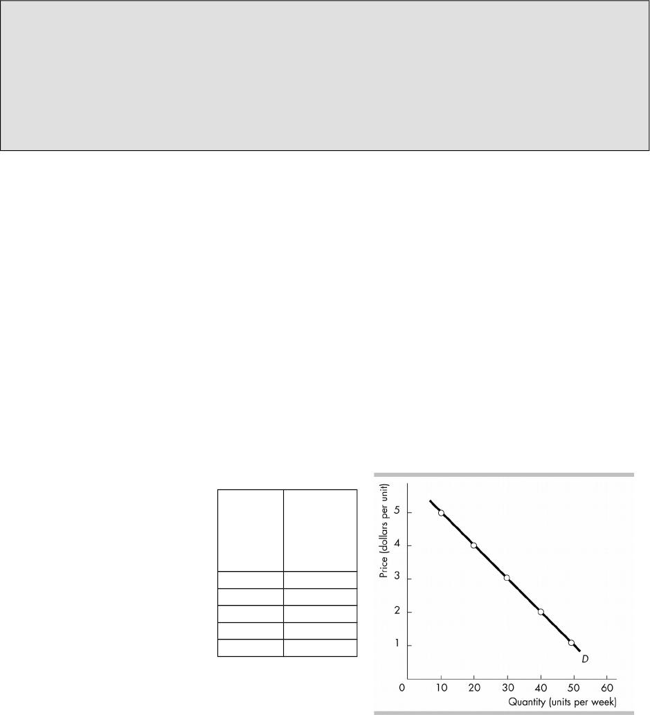
Demand Curve and Demand Schedule
The demand for a
good refers to the
entire relationship
between the price of
the good and the
quantity demanded
of the good. The
table gives a
demand schedule.
© 2016 Pearson Education, Inc.
Price
(dollar
s per
unit)
Quantit
y
demand
ed
(units)
1 50
2 40
3 30
4 20
5 10
A demand curve shows the relationship between the quantity demanded of a good
and its price when all other in4uences on consumers’ planned purchases remain the
same. The gure illustrates the demand curve resulting from the demand schedule.
The demand curve is a willingness-to-pay curve—for each quantity, the price along
the demand curve is the highest price a consumer is willing to pay for that unit of
output which means that a demand curve is a marginal benet curve.
Of the hundreds of classroom experiments that are available today, very few are worth the
time they take to conduct. The classic demand–revealing experiment is one of the most
productive and worthwhile ones. Bring to class two bottles of ice-cold, ready-to-drink Mt.
Dew, bottled water, or sports drink. (If your class is very large, bring six bottles). Tell the
students that you have these drinks and ask them to indicate if they would like one. Most
hands will go up. Tell the class that you are going to sell them to the high bidder. Tell them
that this auction is real. The winner will get the drink and will pay. Ask for a show of hands
of those who have some cash and can a-ord to buy a drink. Explain that these indicate an
ability to buy but not a denite plan to buy. Now begin the auction. Appoint a student to
count hands (more than one for a big class). Begin at a low price: say 10¢ a bottle and
count the number willing to buy. Raise the price in 10¢ increments and keep the tally of the
number who are willing to buy at each price. When the number willing to buy equals the
number of bottles you have for sale, do the transactions. (If you make a prot, and you
might do so, tell the students that the prot, small though it is, will go the department fund
for undergraduate activities—and deliver on that promise.) Now use the data to make a
demand curve for Mt. Dew (or other drink) in your classroom today. You can easily
emphasize the law of demand. And, now that you have a demand curve, you can do some
thought experiments that will shift it. Ask: How would this demand curve have been
di-erent if the temperature in the classroom was 10 degrees higher/lower? How would this
demand curve have been di-erent if half the class was sick and absent today? How would
this demand curve have been di-erent if there was a Coke machine right in the classroom?
A Change in Demand (Demand Shifters)
When any factor that in4uences buying plans other than the price of the good
changes, there is a change in demand and the demand curve shifts. An increase in
demand shifts the demand curve rightward and a decrease in demand shifts the
demand curve leftward. Six factors change demand:
Prices of Related Goods: A substitute is a good that can be used in place of
another good (tea and co-ee) and a complement is a good that is used in
conjunction with another good. (sugar and co-ee). A rise in the price of a
substitute or a fall in the price of a complement increases the demand for the
good.
Expected Future Prices: If the price of a good is expected to rise in the future, the
demand for the good today increases.
Income: A normal good is one for which demand increases as income increases;
an inferior good is one for which demand decreases as income increases.
Expected Future Income and Credit: When expected future income increases,
demand today increases. When credit becomes easier to obtain, demand
increases.
Population: The larger the (relevant) population, the greater the demand.
Preferences: Preferences are an
individual’s attitudes toward goods and
services. If people “like” a good more, the
demand for it increases.
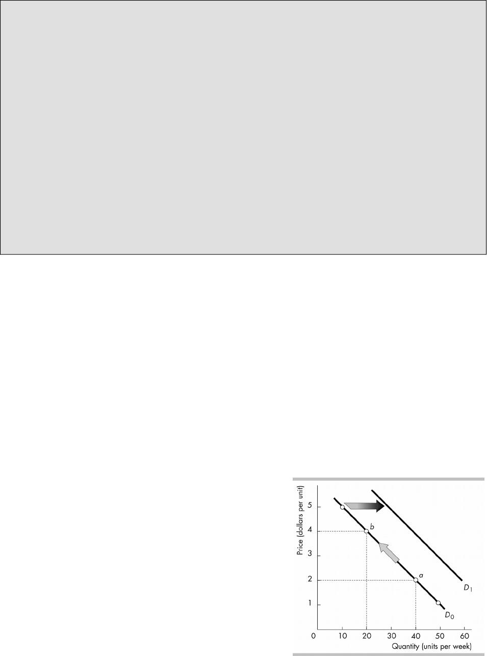
A Change in the Quantity Demanded Versus a
Change in Demand
A change in price results in a movement along
the demand curve, which is change in the
© 2016 Pearson Education, Inc.
2 2 C H A P T E R 3
quantity demanded. A change in other factors shifts the demand curve, which is a
change in demand.
In the gure, the movement along demand curve D0 from point a to point b as a
result of the price rising from $2 to $4 is a change in the quantity demanded. The
shift of the demand curve from D0 to the new demand curve D1 is a change in
demand.
II. Supply
The price of a good or service a-ects the quantity rms plan to sell. The quantity
supplied of a good or service is the amount that rms plan to sell during a given
time period at a particular price.
The law of supply states that other things remaining the same, the higher the
price of a good, the greater is the quantity supplied; and the lower the price of a
good, the smaller the quantity supplied. The law of supply occurs because an
increase in the quantity of a good produced results in an increase in its marginal
cost. So the price must rise in order to induce rms to increase the quantity they
produce.
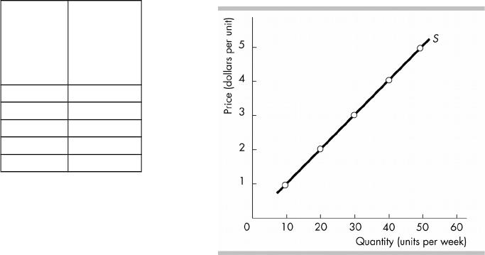
Supply Curve and Supply Schedule
The supply of a good
refers to the entire
relationship
between the price
of the good and
the quantity
supplied of the
good. The table
gives a supply
schedule.
A supply curve
shows the relationship between the quantity
supplied of a good and its price when all
other in4uences on producers’ planned sales
remain the same. The gure illustrates the
supply curve resulting from the supply
schedule.
The supply curve is a minimum-supply-price curve—for each quantity, the price
along the supply curve is the lowest price a producer must receive in order to
produce that unit of output which means that a supply curve is a marginal cost
curve.
A Change in Supply (Supply Shifters)
When any factor that in4uences selling plans other than the price of the good
changes, there is a change in supply and the supply curve shifts. An increase in
supply shifts the supply curve rightward and a decrease in supply shifts the supply
curve leftward. Six factors change supply:
Prices of Productive Resources: If the price of a resource used to produce the
good rises, the supply of the good decreases.
Prices of Related Goods Produced: A substitute in production is a good that can
be produced using the same resources and a complement in production is a good
that must be produced with the initial good. A fall in the price of a substitute in
production or a rise in the price of a complement in production increases the
supply of the good.
Expected Future Prices: If the price of a good is expected to rise in the future, the
supply of the good today decreases.
Number of Suppliers: If the number of suppliers increases, the supply increases.
© 2016 Pearson Education, Inc.
Price
(dollar
s per
unit)
Quantit
y
supplie
d
(units)
1 10
2 20
3 30
4 40
5 50
D E M A N D A N D S U P P LY 2 3
Technology: Technology refers to the ways in which factors of production are used
to produce a good. A technological advance increases the supply of a good.
The State of Nature: The state of nature includes all natural forces that in4uence
supply. Bad weather or an earthquake decreases the supply of a good.
© 2016 Pearson Education, Inc.
2 4 C H A P T E R 3
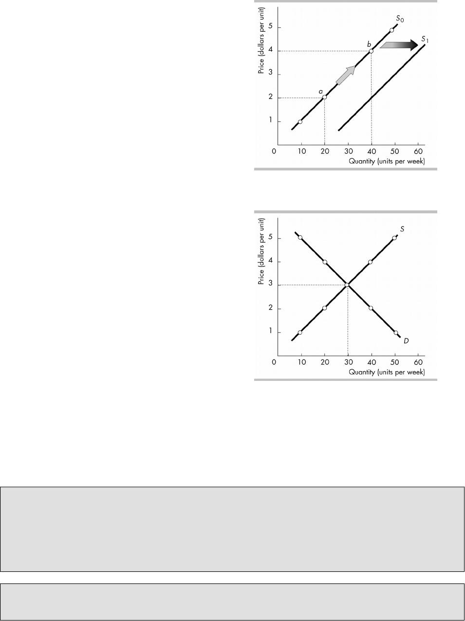
A Change in the Quantity Supplied Versus a
Change in Supply
A change in price results in a movement
along the supply curve, which is change in
the quantity supplied. A change in
other factors shifts the supply curve,
which is a change in supply.
In the top gure, the movement along
supply curve S0 from point a to point b as a
result of the price rising from $2 to $4 is a
change in the quantity supplied. The shift of
the supply curve from S0 to the new
supply curve S1 is a change in supply.
III. Market Equilibrium
An equilibrium is a situation in which
opposing forces balance.
The equilibrium price is the price at
which the quantity demanded equals the
quantity supplied. The equilibrium
quantity is the quantity bought and sold at
the equilibrium price. In the gure, the
equilibrium price is $3 and the
equilibrium quantity is 30 per week.
Price as a Regulator and Price Adjustments
The price of a good regulates the
quantities demanded and supplied.
Shortage: If the price is below the
equilibrium price, consumers plan to buy
more than rms plan to sell. A shortage
results, which forces the price higher, toward the equilibrium price. In the gure,
there is a shortage at any price below $3 and so the price is forced higher, toward
the equilibrium price.
Surplus: If price is above the equilibrium, rms plan to sell more than consumers
plan to buy. A surplus results, which forces the price lower, toward the equilibrium
price. In the gure, there is a surplus at any price above $3 and so the price is forced
lower, toward the equilibrium price.
The price continues to adjust until the quantity supplied equals quantity demanded.
To help students have a base of knowledge from which build tell them to memorize “Home
Base”—the basic Supply and Demand curves showing an initial starting position with
proper labels on the axis’ and an initial equilibrium, P0 and Q0 on the axis at the
intersection of the two curves. “Home Base” provides them a starting place for every story
problem they face. Then as you work through examples, be sure to ask them what “shifter”
is changing. This procedure will keep them using the economic tool rather than just going
with a gut feeling.
The magic of market equilibrium and the forces that bring it about and keep the market
there need to be demonstrated with the basic diagram, with intuition, and, if you’ve already
used the demand experiment outlined above, with hard evidence in the form of the class
© 2016 Pearson Education, Inc.
D E M A N D A N D S U P P LY 2 5
activity. Using the experiment is straightforward. Start by explaining that in that market,
the supply was xed (vertical supply curve) at the quantity of bottles that you brought to
class. The equilibrium occurred where the market demand curve (demand by the students)
intersected your supply curve. Point out that the trades you made in your little economy
made both buyers and sellers better o-.
Back in the dim mists of time, circa 1870 or so, economists struggled to understand if it was
the supply or the demand that determined the price and quantity of a good. Nowadays we
know that these e-orts were misguided. To borrow from the great economist Alfred
Marshall, demand and supply curves are like the blades on a pair of scissors. It does not
make sense to ask which blade does the cutting because the cutting takes both blades and
occurs at the intersection of the two blades. Likewise, it takes both the demand and supply
to determine the price and quantity and the price and quantity are determined at the
intersection of the demand and supply curves.
IV. Predicting Changes in Price and Quantity
The demand and supply model can be used to determine how changes in factors a-ect a
good’s price and quantity.
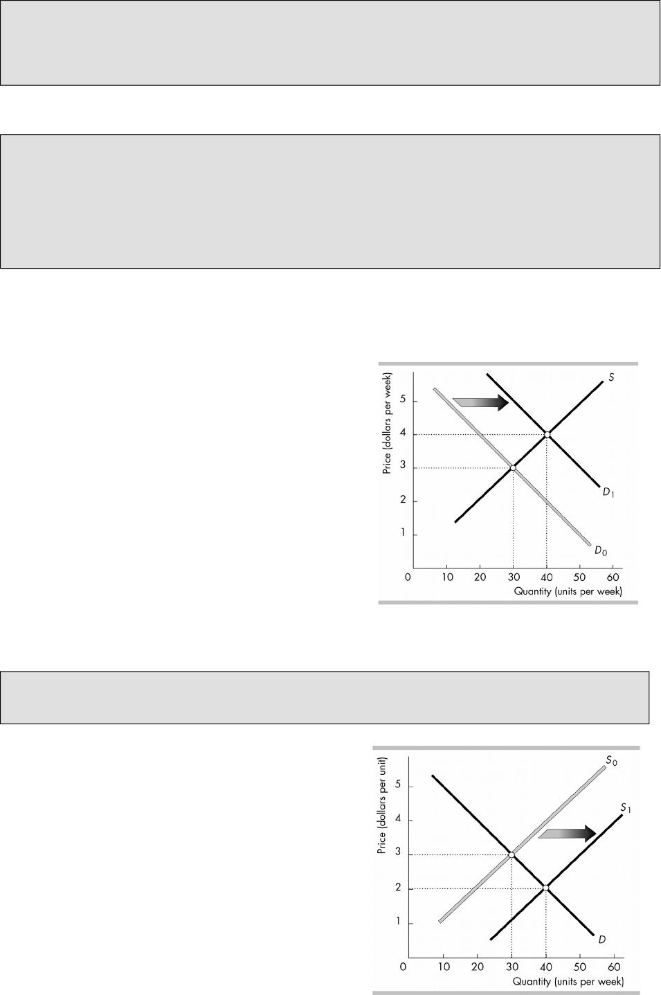
A Change In Demand
If the demand for a good or service
increases, the demand curve shifts
rightward. As a result, the equilibrium price
rises and the equilibrium quantity
increases.
If the demand for a good or service
decreases, the demand curve shifts
leftward. As a result, the equilibrium price
falls and the equilibrium quantity
decreases.
Supply does not change and the supply
curve does not shift. Instead there is a
change in the quantity supplied and a
movement along the supply curve.
The gure illustrates an increase in
demand. In the gure the demand curve
shifts from D0 to D1. As a result, the equilibrium price rises from $3 to $4 and the
equilibrium quantity increases from 30 to 40. The supply curve does not shift; there
is, however, a movement along the supply curve.
An Economic in the News feature discusses the factors that have led to higher college
tuition. Because enrollment has also increased, the analysis concludes that increases in
demand are the factor that has created the higher tuition.
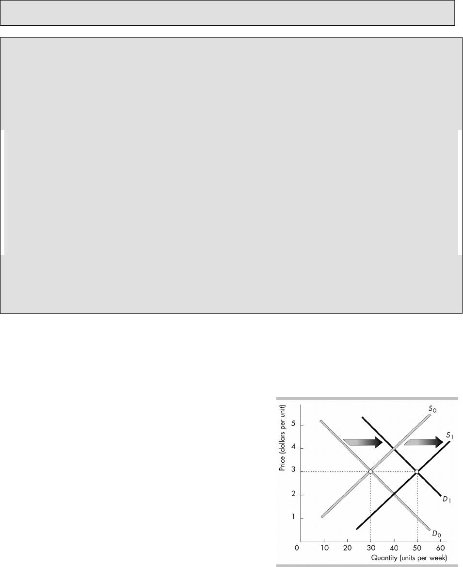
A Change In Supply
If the supply of a good or service
increases, the supply curve shifts
rightward. As a result, the equilibrium
price falls and the equilibrium quantity
increases.
© 2016 Pearson Education, Inc.
2 6 C H A P T E R 3
If the supply of a good or service decreases, the supply curve shifts leftward. As a
result, the equilibrium price rises and the equilibrium quantity decreases.
Demand does not change and the demand curve does not shift. Instead there is a
change in the quantity demanded and a movement along the demand curve.
The gure illustrates an increase in supply. In the gure the supply curve shifts from
S0 to S1. As a result, the equilibrium price falls from $3 to $2 and the equilibrium
quantity increases from 30 to 40. The demand curve does not shift; there is,
however, a movement along the demand curve.
An Economic in the News explores the factors that led to a fall in the price of co-ee. The
analysis concludes that a bumper crop of co-ee lies behind the fall in price.
The whole chapter builds up to this section, which now brings all the elements of demand,
supply, and equilibrium together to make predictions. Students are remarkably ready to
guess the consequences of some event that changes either demand or supply or both. They
must be encouraged to work out the answer and draw the diagram. Explain that the way to
answer any question that seeks a prediction about the e-ects of some event(s) on a market
has ve steps. Once you have already worked an example or two, walk them through the
steps and have one or two students work some examples in front of the class. The ve steps
are:
1. Draw a demand-supply diagram and label the axes with the price and quantity of the
good or service in question.
2. Think about the event(s) that you are told occur and decide whether they change
demand, supply, or both demand and supply.
3. Determine if the events that change demand or supply bring an increase or a decrease.
4. Draw the new demand curve and supply curve on the diagram. Be sure to shift the
curve(s) in the correct direction—leftward for decrease and rightward for increase. (Lots
of students want to move the curves upward for increase and downward for decrease—
this view works ok for demand but is exactly wrong for supply. So emphasize the
left-right shift.)
5. Find the new equilibrium and compare it with the original one.
It is critical at this stage to return to the distinction between a change in demand (supply)
and a change in the quantity demanded (supplied). You can now use these distinctions to
describe the e-ects of events that change market outcomes. At this point, the students
know enough for it to be worthwhile emphasizing the magic of the market’s ability to
coordinate plans and reallocate resources.
Demand and Supply Change in the Same Direction
If both the demand and the supply of a good or service increase, both the demand
and supply curves shift rightward. The quantity unambiguously increases but the
e-ect on the price is ambiguous.
If the increase in demand is greater than the increase in supply, the price rises.
If the increase in demand is the same size as the increase in supply, the price
does not change.
If the increase in demand is less than the
increase in supply, the price falls.
If both the demand and the supply of a good
or service decrease, both the demand and
supply curves shift leftward. The quantity
unambiguously decreases but the e-ect on
the price is ambiguous.
© 2016 Pearson Education, Inc.
D E M A N D A N D S U P P LY 2 7
If the decrease in demand is greater than the decrease in supply, the price falls.
If the decrease in demand is the same size as the decrease in supply, the price
does not change.
If the decrease in demand is less than the decrease in supply, the price rises.
The gure illustrates an increase in both demand and supply. In the gure the
demand curve shifts from D0 to D1 and the supply curve shifts from S0 to S1. The
shifts are the same size, so the equilibrium price does not change and the
equilibrium quantity increases from 30 to 50.
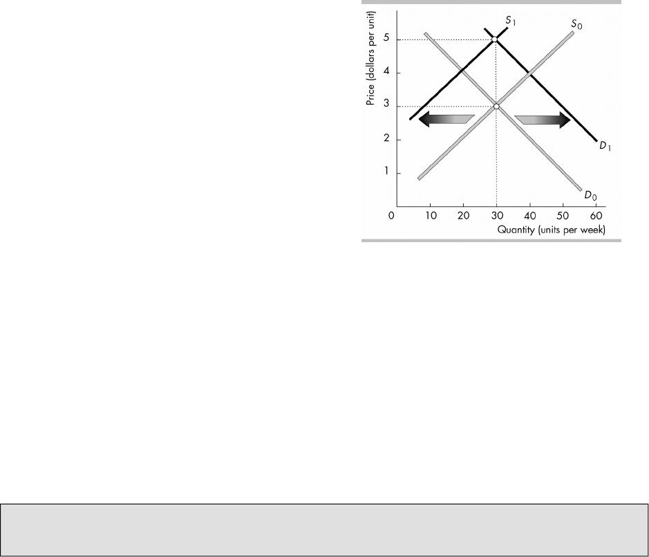
Demand and Supply Change in the Opposite
Directions
If the demand increases and the supply
decreases, the demand curve shifts
rightward and the supply curve shifts
leftward. The price unambiguously rises
but the e-ect on the quantity is
ambiguous.
If the increase in demand is greater
than the decrease in supply, the
quantity increases.
If the increase in demand is the same
size as the decrease in supply, the
quantity does not change.
If the increase in demand is less than
the decrease in supply, the quantity
decreases.
If the demand decreases and the supply increases, the demand curve shifts leftward
and the supply curves shifts rightward. The price unambiguously falls but the e-ect
on the quantity is ambiguous.
If the decrease in demand is greater than the increase in supply, the quantity
decreases.
If the decrease in demand is the same size as the increase in supply, the
quantity does not change.
If the decrease in demand is less than the increase in supply, the quantity
increases.
The gure illustrates an increase in demand and a decrease in supply. In the gure
the demand curve shifts from D0 to D1 and the supply curve shifts from S0 to S1. The
shifts are the same size, so the equilibrium quantity does not change and the
equilibrium price rises from $3 to $5.
The Economic in the News explores the market for bananas. A disease that damages
banana crops has spread from Southeast Asia to the Middle East. The disease has
decreased the supply of bananas, resulting in the price rising and quantity decreasing.
© 2016 Pearson Education, Inc.
2 8 C H A P T E R 3