
W H AT I S E C O N O M I C S ? 1 9 7
T h e B i g P i c t u r e
Where we have been:
Chapter 18 uses the productivity and cost denitions and concepts introduced
in Chapter 10 and the conditions for maximum prot introduced in Chapter 11.
It builds on these concepts to explain value of marginal product and to show
how factor markets work.
Where we are going:
Chapter 18 explores the workings of factor markets and the resulting
distribution of income. The labor, capital, and natural resource markets are
introduced here and Chapter 19 studies the implications of factor market
equilibrium for the distribution of income and trends in the distribution.
N e w i n t h e Tw e l f t h E d i t i o n
The material in the chapter is largely unchanged from the previous edition. The
focus remains on the job market and the case studies and applications have been
updated. A new Worked Problem section has been added. The Worked Problem
shows the students how to calculate the marginal product of labor and the value
of marginal product. It then demonstrates how to use the results to maximize
prot and how the prot-maximizing quantity of labor changes when the age rate
changes. To include the new Worked Problem without lengthening the chapter,
some problems have been removed from the Study Plan Problem and
Applications. These problems are in the MyEconLab and are called Extra Problems.
18MARKETS FOR
FACTORS OF
PRODUCTION
C h a p t e r
197
L e c t u r e N o t e s
Markets for Factors of Production
Firms choose the quantities of factors they demand in order to maximize their prot.
Households choose the quantities of factors they supply.
The interaction of demand and supply determines factor prices.
I. The Anatomy of Factor Markets
The four factors of production are labor, capital, land (natural resources), and
entrepreneurship.
Labor services are traded in the labor market. The price of labor is the wage rate.
Most labor services are traded on a job contract.
Capital goods are traded in goods markets. Capital services are traded in rental
markets. The services of capital that a rm owns have an implicit price that arises
from depreciation and interest costs. Firms that buy capital and use it themselves
are implicitly renting the capital to themselves.
The price of the services of land is a rental rate. Nonrenewable natural
resources are resources that can be used only once.
Entrepreneurs receive the prot (or loss) that results from their business decisions
and their services are not traded in markets.
Looking back Before you jump into the content of this chapter, provide your students with
some context and perspective.
1. Recall the big issues of microeconomics discussed in Chapter 1. Point out that the
course so far has addressed the rst two questions: “What?” and “How?” and that
you’re now going to address how markets determine the answer to the third question:
“For whom?”
2. Spend a minute or two reviewing the course so far. Point out that Chapters 3–7,
demand and supply and its extensions and applications studied the @ows of goods and
services from rms to households. Chapters 8 and 9 studied the choices of households.
Chapters 10–15 studied the choices of rms. Now, we’re going to study the @ow of
goods and services from rms to consumer households in the product market and the
@ow of factors of production from households to rms in the factor markets.
3. Understanding choices at the margin, demand and supply, and market forces that
bring equilibrium and coordinate activity to produce eCciency are all used in this
chapter. Emphasize the power of the economic tools that the students already know
and the payoD from keeping on top of the entire course.
II. The Demand for a Factor of Production
The Value of Marginal Product
The demand for a factor of production
is called a derived demand because
it is derived from the demand for the
goods and services produced by the
factor.
The value to the rm of hiring one
more unit of a factor of production is
called the factor’s value of marginal
© 2016 Pearson Education, Inc.
Labor
(hours
per
day)
Output
(units
per
day)
Marginal
product
of labor
(units per
day)
Value of
margina
l
product
(dollars)
200 1,000
20 140
300 3,000
10 70
400 4,000
5 35
500 4,500

W H A T I S E C O N O M I C S ? 1 9 9
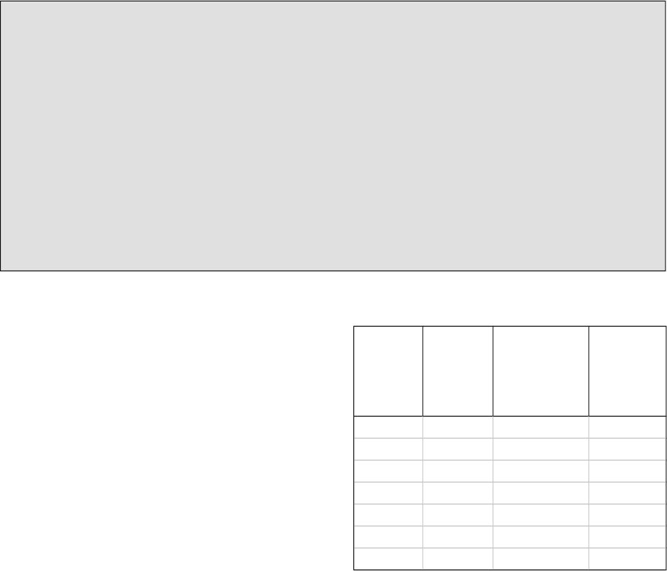
product. It is equal to the price of a unit of output multiplied by the marginal
product of the factor of production:
VMP = P MP
The table shows the calculation of the VMP for a rm whose output has a price of $7
per unit.
A Firm’s Demand for Labor
The rm hires the quantity of labor that maximizes its prot by comparing the value
of one more worker (the VMP) to the cost of employing one more worker, the wage
rate.
As more labor is employed, the MP diminishes (as shown in the table above). So as
more labor is employed, the VMP diminishes.
If VMP of labor exceeds the wage rate, the rm increases its prot by employing one
more worker; if VMP is less than the wage rate, the rm increases its prot by
employing one less worker; and, if VMP equals the wage rate, the rm is employing
the prot-maximizing quantity of labor.
A Firm’s Demand for Labor Curve
The value of marginal product curve is the rm’s labor demand curve.
Because the VMP of labor diminishes as the quantity of labor employed increases,
the demand curve for labor is downward sloping.
The prot-maximizing level of inputs implies the prot-maximizing level of
output. If you wish to go beyond the analysis in the book, you can take a bit of time to
show your students the basic math of the equivalence of the two conditions for maximum
prot—MR = MC and W = VMP—and give them a good intuitive grasp of what is going on.
There are six steps:
1. The cost of producing one more unit, MC, equals the cost of one more worker, W,
divided by that worker’s marginal product, MP. That is: MC = W/MP.
2. The revenue from selling one more unit, MR, equals the revenue from hiring one more
worker, VMP, divided by that worker’s marginal product, MP. That is: MR = VMP/MP.
3. Setting these two equations side by side: MC = W/MP and MR = VMP/MP is a tiny step to
see that MC = MR implies W = VMP.
4. Just write MC = MR implies W/MP = VMP/MP; multiply by MP and W = VMP.
5. Now put in some numbers to make the student who freezes on symbols more
comfortable.
6. Finally, just talk about what the equations mean. Explain that the marginal worker
costs $x and generates a revenue of $x, so that worker is just worth hiring. Hiring one
more worker costs $x but generates less than $x in revenue, so is not worth hiring.
Hiring one fewer worker saves $x but forgoes more than $x in revenue, so prot falls.
Go on to point out that one unit of output produced by the marginal worker sells for $p
and it costs $x/MP, which equals marginal cost.
Changes in a Firm’s Demand for Labor
Three factors can change the demand for labor and shift the labor demand curve:
If the price of the rm’s output changes, the VMP changes, which changes the
demand for labor. An increase in the price of the output increases the demand for
labor and shifts the demand curve rightward.
If the prices of other factors of production change, in the long run the demand for
labor changes. An increase in the price of a substitute factor leads the rm to
increase the demand for labor.
199

If a change in technology increases the productivity of one type of labor, the demand
for this labor increases and the demand curve shifts rightward.
III. Labor Markets
A Competitive Labor Market
The market demand for labor is determined by adding together the quantities of
labor demanded by all the rms in the market at each wage.
The market supply of labor is derived from the supply of labor decisions made by
individual households.
Aren’t households demanders? Point out that in the labor market, the tables have been
turned compared to the goods and services market. The household that is on the demand
side of the markets for consumer of goods and services is now on the supply side of the
market.
A person’s reservation wage is the lowest wage rate for which the person is willing to
supply labor. As the wage rate rises above the reservation wage, there is a
substitution eDect and an income eDect. The substitution eDect occurs because a
higher wage rate increases the opportunity cost of leisure, which increases the
quantity of labor supplied. The income eDect occurs because an increase in the
wage rate increases the person’s income and so increases the demand for leisure,
which decreases the quantity of labor supplied.
At lower wage rates, the substitution eDect dominates the income eDect, so a rise in
the wage rate increases the quantity of labor supplied. At higher wage rates, the
income eDect dominates the substitution eDect, so a rise in the wage rate decreases
the quantity of labor supplied and the supply of labor curve bends backward.
What’s your reservation wage? Ask the students if they would be willing to work 40
hours each week at a wage rate of $20 per hour (which is about $40,000 per year). Next,
ask them whether they would increase their labor supplied to 48 hours per week if they
could earn $40 per hour (about $80,000 per year, if working 40 hours per week). Most
students would be willing to work more hours per week at this wage rate. Then ask them
how many hours per week they would work if they were paid $10,000 per hour. In this
case, working only one day per week would garner them about $8 million per year, leaving
the remaining six days of each week to enjoy their high income. Many would not be willing
to continue working 48 hours a week, thereby creating a backward-bending supply of labor
curve.
The supply of labor increases (shifts rightward) when the adult population increases
and when capital and technology used in the home increase.
Labor market equilibrium determines the wage rate and employment.
Comparing competitive output markets with competitive input markets. Just as
the perfectly competitive rm in the market for a good or service is a price taker in that
market, so the individual household in a perfectly competitive factor market is a price
taker. Also, the rm that buys the services of the factor of production is a price taker in a
perfectly competitive factor market. Even in the market for land, which is in perfectly
inelastic supply, the individual landowner faces a perfectly elastic demand for his or her
land.

W H A T I S E C O N O M I C S ? 2 0 1
Di%erences and Trends in Wage Rates
DiDerences in demand and supply across labor markets make wage rates unequal.
The highest wage rates are earned in markets where the value of marginal product
is high and where few people have the ability and training for the job.
Because the value of marginal product increases over time as new capital and new
technologies increase labor productivity, wage rates also increase over time.
Wage inequality has increased recently with high wage rates increasing more
rapidly than low wage rates. Some low wage rates have stagnated or fallen. The
new information technologies increased the productivity and wage rates of already
high-paid workers. Globalization has brought increased competition for low-skilled
workers and lowered the wages of already low-paid workers.
An Economics in Action case has been updated with current Bureau of Labor Statistics data
on U.S. wages. The diDerence between median and mean income is highlighted as more
Americans earn less than the average income. The application also notes that higher than
average wage jobs typically require college and post graduate degrees.
An Economics in the News case considers how college majors aDect job prospects.
Biomedical engineering earns the top rating for starting median salary combined with
anticipated job growth. With both demand and supply increasing, the number of
biomedical engineers is expected to grow 60 percent between now and 2020. The case
takes students through the analysis of the changes in demand and supply and helps them
understand why both the number of jobs and salaries are expected to increase.
A Labor Market with a Union
A labor union is an organized group of workers that aims to increase the wage rate and
in@uence other job conditions. The text analyzes how unions impact the labor market
equilibrium for union workers and how this impacts nonunion workers.
To reach their goals, unions attempt to restrict the quantity of labor available for the
rm to employ (shifting the labor supply curve leftward).
Unions also attempt to in@uence the demand for labor and to increase the demand
for labor (shifting the labor demand curve rightward) with the following strategies:
Increase the marginal product of union members to increase the demand for
their labor.
Encourage import restrictions to increase the demand for union-made U.S.
products.
Support minimum wage laws to raise the cost of non-union low-skilled labor.
Support immigration restrictions to decrease the supply of competitive labor.
In equilibrium, if a union decreases the supply of labor, there will be fewer jobs at
higher wages. If it is able to also increase the demand for union labor, this will
further increase wages and oDset some of the decrease in employment. The market
for nonunion labor will also be eDected workers unable to get union jobs increase the
supply.
Monopsony in the Labor Market
A monopsony is a market in which there is a single buyer.
For a monopsony, the marginal cost of labor exceeds the wage rate because the
monopsony faces an upward-sloping labor supply curve. To attract one more worker,
the monopsony must oDer a higher wage rate, and it must pay this higher wage rate
to all its workers.
201
Example: The idea that the marginal cost of labor is somehow diDerent from the wage
rate is often confusing for students. Be sure to go through the intuition and the math
calculations for the marginal cost of labor several times. As in the table below, if
employment rises from 200 to 300 hours per day, the wage rate will rise from $3 to $6. The
total cost of labor rises from $600 to $1,800, a diDerence of $1,200. The change in total
cost divided by the change in employment will be $1,200/100 = $12. Intuitively, all 200
hours of labor were earning a wage of $3 per hour until the next 100 hours of labor were
employed. To entice those units of labor to supply their services, the wage rate rose to $6
for all 300 units of labor. As a result, the rm pays $6 for the new 100 hours of labor, and
pays an additional $3 for the 200 hours of labor it was previously employing. That’s $600
for the new 100 units of labor and an additional $600 for the wage increase paid to the
original 200 units of labor, for a marginal cost of labor equal to $1,200/100 = $12 again.
What about “wage discrimination”? Monopolies faced a downward-sloping demand
curve for their output, resulting in a marginal revenue curve that was below the demand
curve. To sell more output, monopolies had to lower the price. The story for monopsony is
similar. Because a monopsony faces an upward-sloping supply curve for labor, to hire more
labor, monopsonies have to raise the wage, resulting in a marginal cost of labor curve that
is above the labor supply curve. Some of your especially attentive students will remember
that marginal revenue and demand were the same when the rm could practice perfect
price discrimination. In the basic model of monopsony, we’re assuming there’s no “wage
discrimination.” Every worker is paid the same wage, just as every customer in a
single-price monopoly is charged the same price.
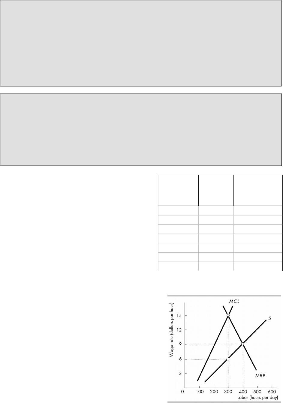
The rst two columns of the table show
the labor supply schedule and the last
column has the marginal cost of labor,
MCL, schedule. The MCL curve is upward
sloping and lies above the labor supply
curve.
To maximize its prot, a monopsony hires
the quantity of labor where its MCL is
equal to VMP and then pays the wage
rate necessary to attract that quantity of
labor. In the gure, the monopsony
employs 300 hours of labor per day and
pays a wage rate of $6 per hour.
A monopsony hires less labor and pays a
lower wage rate than it would if it were
operating in a competitive labor market. In
the gure, in a competitive labor market 400
hours of labor would be employed and the
wage rate would be $9 per hour.
Labor
(hours per
day)
Wage
rate
(dollars
per hour)
Marginal cost
of labor
(dollars per
hour)
200 3
12
300 6
18
400 9
24
500 12

W H A T I S E C O N O M I C S ? 2 0 3
A Union and a Monopsony
If a union, a monopoly seller of labor services, faces a monopsony buyer of labor
services, the situation is called bilateral monopoly. In a bilateral monopoly, the
wage rate is determined by bargaining and depends on the costs that each party
can in@ict on the other if they fail to agree upon a wage rate.
Examples of bilateral monopoly: Have the students consider the relationship between
professional team owners (NBA, NFL, etc.) and the players who work for these owners.
Such markets are classic examples of bilateral monopoly. Team owners operate a legal
cartel and maintain strict rules for hiring labor (drafting and trading players) that prevent
most of the competition among team owners who might want to sign the same player. So
the owners are close to a monopsony. The best players with uniquely talented skills cannot
be duplicated in the short run, so these players have a monopoly on their skills. The
resulting bilateral monopoly equilibrium is such that player’s wages in general are high
compared to most all other professions. This observation might surprise the students
because it suggests that bargaining position of the players is greater than that of the
owners.
Monopsony and Minimum Wages
The imposition of a minimum wage in a monopsony labor market might increase
both the wage rate and employment. The minimum wage makes the supply of labor
perfectly elastic over some range of employment. Over this range the supply curve
is horizontal and the MCL of an additional employee equals the minimum wage rate.
If this part of the supply curve of labor intersects the monopsony’s VMP curve, the
minimum wage increases both the quantity of labor employed by the monopsony
and the wage rate paid by the monopsony. The wage rate equals the minimum wage
rate.
The At Issue case presents the argument over whether monopolies are always bad,
focusing on the NCAA. Robert Barro argues that the NCAA monopoly hurts the market for
college athletics. Richard McKenzie and Dwight Lee argue that the NCAA monopoly has
helped college athletics.
203