
T h e B i g P i c t u r e
Where we have been:
Chapter 12 on perfect competition has shown the student how rms make
output and pricing decisions under competitive market assumptions. Chapter
13 explains how a rm with monopoly power makes those same decisions.
Chapter 13 evaluates the eciency of monopoly relative to perfect
competition. It also covers regulation of a natural monopoly.
Where we are going:
Chapter 14 describes rms and industries in monopolistic competition.
Chapter 15 lls in the middle of the spectrum with a study of oligopoly. The
material discussing a monopoly’s downward-sloping demand curve and
resulting downward sloping marginal revenue curve is used in the next
chapter in the context of a rm in monopolistic competition. The result that a
monopoly can earn an economic prot is used in Chapter 15 as the
explanation why oligopolistic rms want to collude to raise their prices and
decrease the quantity they produce.
N e w i n t h e Tw e l f t h E d i t i o n
The chapter opening and a new Economics in the News case at the end of the
chapter look at Google’s success in the market. Is its dominance in search serving
the market and social interests or violating anti-trust law? A new Worked Problem
section has been added. The Worked Problem gives the students the demand and
cost schedule for a monopoly. It then shows the students how to calculate the
prot-maximizing price, quantity, economic prot, and producer surplus if the rm
is a single-price monopoly. Then it demonstrates to the students the
prot-maximizing quantity, economic prot, and producer surplus if the rm can
perfectly price discriminate. To include the new Worked Problem without
lengthening the chapter, some problems have been removed from the Study Plan
Problem and Applications. These problems are in the MyEconLab and are called
Extra Problems.
© 2016 Pearson Education, Inc
13 MONOPOLY
C h a p t e r
M O N O P O LY 143

L e c t u r e N o t e s
Monopoly
A monopoly is a market with a single rm that is protected by barriers to entry.
A monopoly maximizes its prot by producing where MR = MC and then using its
demand curve to set its price.
Price-discriminating monopolies charge a higher price to customers with a higher
willingness to pay.
Compared to a competitive market, a monopoly sets a higher price, produces a
smaller quantity, and converts consumer surplus into economic prot.
Natural monopolies can be regulated by the government.
I. Monopoly and How It Arises
A monopoly is a rm that produces a good or service for which no close substitute exists
and which is protected by a barrier that prevents other rms from selling that good or
service.
How a Monopoly Arises
A monopoly has two key features:
No Close Substitutes: There are no close substitutes for the good or service.
Barriers to Entry: A constraint that protects a rm from potential competition is
called a barrier to entry. There are three types of entry barriers:
Natural barriers to entry create a natural monopoly, which is an industry in
which economies of scale enable one rm to supply the entire market at the
lowest possible cost.
An ownership barrier to entry occurs if one rm owns a signicant portion of a
key resource.
Legal barriers to entry create a legal monopoly, which is a market in which
competition and entry are restricted by the granting of a public franchise (an
exclusive right is granted to a rm to supply a good or service—the U.S. Postal
Service has a public franchise to deliver rst-class mail), a government license
(when the government controls entry into particular occupations, professions and
industries—a license is required to practice law), a patent (an exclusive right
granted to the inventor of a product or service) or a copyright (exclusive right
granted to the author or composer of a literary, musical, dramatic, or artistic
work). In the U.S., patents last twenty years, encouraging innovation and
stimulating invention.
Who has to have a license to produce? There are many examples of government
licensing. Licensing can protect consumers from fraud and abuse, but it can also hurt
consumers by preventing competition from producing an ecient allocation of resources.
Have the students debate the merits of the following licensing arrangements: 1) Doctors
can receive a medical license to practice medicine only by graduating from an
AMA-approved medical program; 2) Lawyers can practice law only after passing an
extensive Bar Exam; 3) Cab drivers in New York City can operate a taxi only if they have
purchased a medallion from the city, of which there are a nite number; 4) Beauticians in
many states cannot operate a beauty parlor without a state certication that requires
training in sanitary practices as well as other courses completely unrelated to their
profession (such as civics and history courses).
© 2016 Pearson Education, Inc
What’s the advantage of patents? Granting an innovator a monopoly to the innovation
increases the incentives to innovate. But the evidence whether monopoly leads to greater
innovation is mixed. Consider the struggle for developing countries with populations
dealing with epidemics such as AIDS. In the developed countries in which they operate,
pharmaceutical companies are granted legal barriers (patents) on their drugs, granting
them a legal monopoly and enabling them to earn a high economic prot once they bring a
new and successful medicine to market. The anticipation of this prot provides the
incentive for these rms to undertake the expensive (currently estimated at approximately
$900 million per approved drug) and risky development of innovative cures for the terrible
diseases aDicting mankind, such as AIDS. However, once the new medicines are made
available, the absence of competition means the price is high, which decreases the use of
these new medicines, especially among the population of the poorer, developing nations
that have been hit the hardest by these diseases. So, once the drug is discovered, the
monopoly creates a deadweight loss but without the economic prot the monopoly brings,
the drug might not have been discovered. There is a tradeoE between current suEerers,
who want a low price, and suEerers in the future, who want new and better medicines
developed.
The Economics in Action case considers how the information age has led to the creation of
new natural monopolies. These rms have high xed costs but almost zero marginal costs.
The rms cited include Google, Microsoft, and Facebook. These same information age
technological changes have hurt other monopolies such as the U.S. Postal Service, with
competition from FedEx, UPS, email, and online payments systems. Local cable television
providers now face competition from satellite and phone companies.
Monopoly Price-Setting Strategies
A single-price monopoly is a rm that sells each unit of its output for the same
price to all its customers.
Price discrimination is the practice of selling diEerent units of a good or service
for diEerent prices. Many rms price discriminate, but not all of them are monopoly
rms.
II. A Single-Price Monopoly’s Output and Price Decision
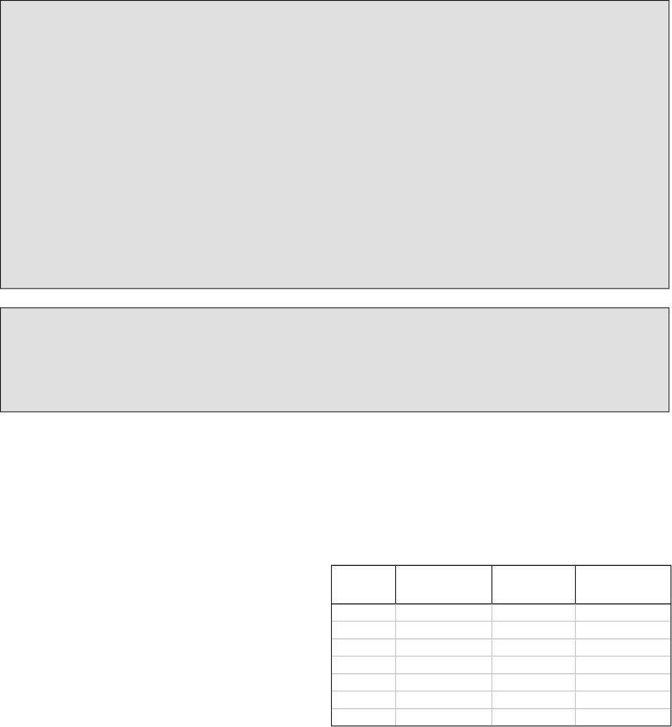
Price and Marginal Revenue
The demand curve facing a
monopoly rm is the market
demand curve. Total revenue (TR)
is the price (P) multiplied by the
quantity sold (Q). Marginal revenue
(MR) is the change in total revenue
resulting from a one-unit increase
in the quantity sold.
The table shows the calculation of
TR and MR.
A key feature of a single-price monopoly is that MR < P at each quantity so the MR
curve lies below the demand curve. MR < P because a single–price monopoly must
lower its price on all units sold to sell an additional unit of output.
© 2016 Pearson Education, Inc
Price
Quantity
demanded
Total
revenue
Marginal
revenue
$4 0 $0
$3
$3 20 $60
$1
$2 40 $80
$1
$1 60 $60
M O N O P O LY 1 4 5
Why is MR below the price? While the formula isn’t dicult, students often have trouble
understanding this concept intuitively. If a rm sells output for $2, why aren’t they getting
$2 of revenue for each unit of output they sell so that marginal revenue is $2? Remind
students that we are assuming that the monopoly charges the same price to all
consumers. As in the table above, if on any given day, every consumer is paying $2 for
output, 40 units are demanded and total revenue is $80. If the monopoly decides it wants
to sell more than 40 units the next day, it must lower the price to do so. The monopoly is
NOT simply lowering the price to $1 for units 41 through 60. Rather, the monopoly lowers
the price on ALL units it will sell the next day. As a result, units 1 through 40 that
customers used to pay $2 for will now be sold for only $1. That’s a loss of $1 on each of
those 40 units for a revenue loss of $40. Part of that revenue loss is oEset by the sales of
units 41 through 60. Since the rm gains $1 in revenue from the sale of each of those
units, there is a revenue gain of $20. A revenue loss of $40 (from lowering prices)
compared with a revenue gain of $20 (from selling more output) generates a net revenue
loss of $20, and (when divided by the change in output from 40 to 60) a marginal revenue
of negative $1. For visual learners, showing these areas of revenue gain and revenue loss
should also help (similar to Figure 13.2 in the text).
Marginal Revenue and Elasticity
If demand is elastic, the MR is positive. A decrease in the price will result in a
proportionately greater increase in quantity, generating an increase in revenue.
If demand is unit elastic (as it is at the midpoint of a linear demand curve), the MR
equals zero. A change in the price will result in a proportionate change in quantity,
generating no change in revenue. If further increase in revenue is not possible from
changing price, this is also the point where revenue is maximized.
If demand is inelastic, MR is negative. A decrease in price will result in a
proportionately smaller increase in quantity, generating a decrease in revenue.
A single-price monopoly never produces in the inelastic part of its demand because
if it did, the rm could increase its total prot by decreasing its output, which would
raise its total revenue and decrease its total cost.
But if a monopoly is the only producer so there are no substitutes, isn’t demand
always inelastic? This question is common. As the only producer of a good, a monopoly
does have some control over the price it charges for output, and students understand that
conceptually. For example, when you go to the movie theater, you know you’re likely to pay
$5 or more for a tub of popcorn, even though you could buy the same amount of popcorn
at the grocery store for $1 or less. Because you’re stuck at the movie theater with
whatever options they oEer, consumers end up paying a higher price. In other words,
because there are fewer substitutes at the theater, demand for popcorn is less elastic.
However, that fact does NOT mean that the demand for popcorn at a movie theater
universally has an elasticity of demand that’s less than one. Even if demand for a
monopoly’s product is fairly inelastic, the demand still has some ranges where elasticity is
greater than one (anywhere above the midpoint on a linear demand curve, for example).
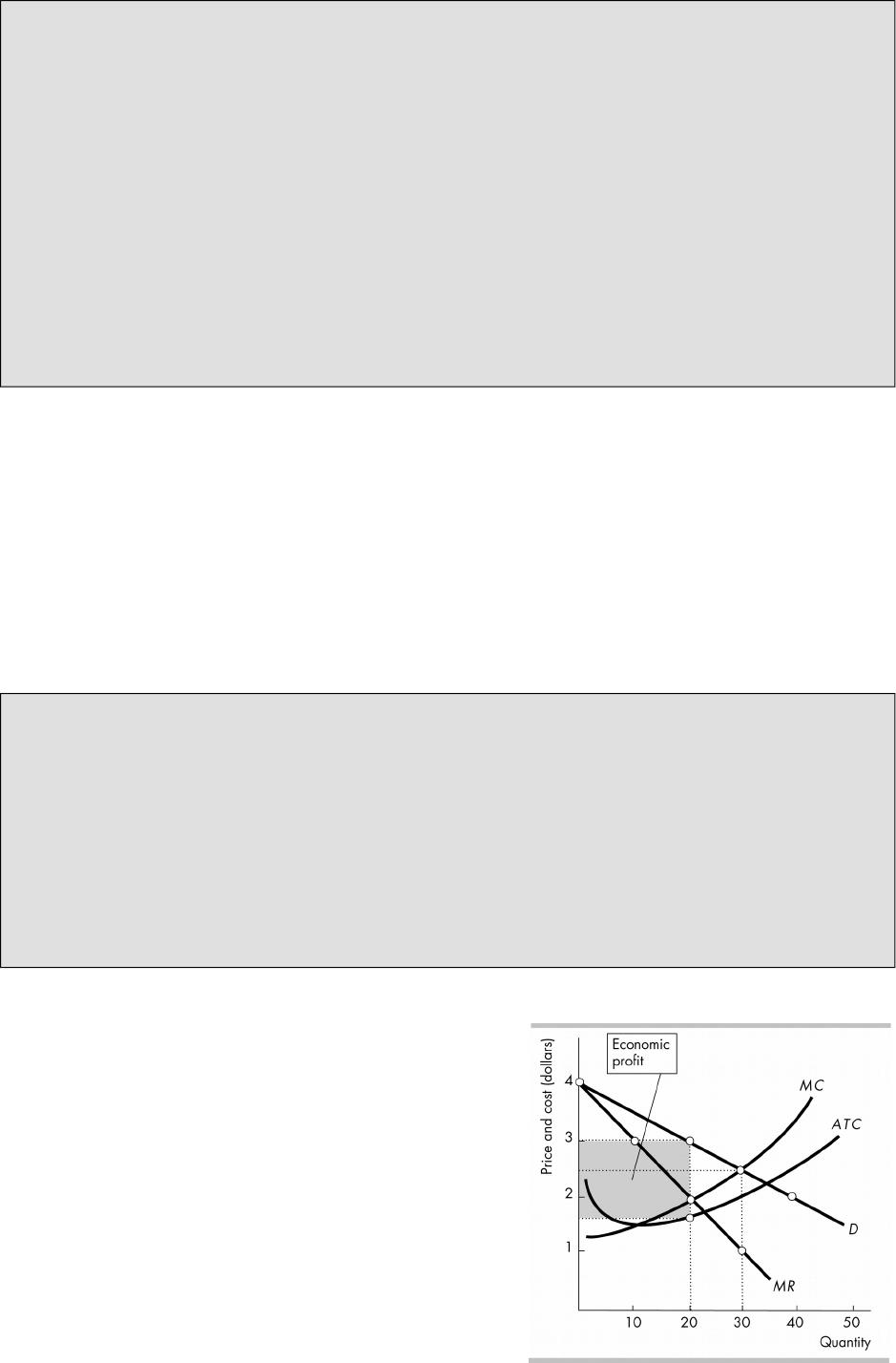
Price and Output Decision
To maximize its prot, a monopoly produces
the level of output where MR = MC. The
monopoly then uses its demand curve to set
the price at the highest price for which it will
be able to sell the quantity it produces. In
the gure, which uses the demand and MR

schedules from the table above, the rm produces 20 units of output and sets a price
of $3 per unit.
The rm makes an economic prot if P > ATC, which is the case for the rm in the
gure. The monopoly can make an economic prot even in the long run because the
barriers to entry protect the rm from competition. However, a monopoly rm is not
guaranteed an economic prot. In the short run and/or long run, it might make zero
economic prot, (P = ATC) or in the short run, it might incur an economic loss
(P < ATC).
Joan Robinson and Paul Samuelson: The classic monopoly diagram provides a good
opportunity to tell your students about the contribution of one of the most brilliant
economists of the 20th century, Joan Robinson. This diagram rst appeared in her book,
The Economics of Imperfect Competition, published in 1933 when she was just 30 years
old.
Women are still not attracted to economics on the scale that they’re attracted to most
other disciplines, so the opportunity to talk about an outstanding female economist
shouldn’t be lost. Joan Robinson was a formidable debater and reveled in verbal battles, a
notable one of which was with Paul Samuelson on one of her visits to MIT. Anxious to make
and illustrate a point, Samuelson asked Robinson for the chalk. Monopolizing the chalk and
the blackboard, the unyielding Robinson snapped, “Say it in words young man.”
Samuelson meekly obeyed. This story illustrates Joan Robinson’s approach to economics:
work out the answers to economic problems using the appropriate techniques of math and
logic, but then “say it in words.” Don’t be satised with formal argument if you don’t
understand it. Your students will benet from this story if you can work it into your class
time.
III. Single-Price Monopoly and Competition Compared
Comparing Price and Output
Perfect Competition: The market demand curve (D) in perfect competition is the
same demand curve that the rm faces in monopoly. The market supply curve (S) in
perfect competition is the horizontal sum of the individual rm’s marginal cost
curves. This supply curve also is the monopoly’s marginal cost curve, so in the gure
above the supply curve is labeled MC. In a competitive market, equilibrium occurs
where the quantity demanded equals the quantity supplied. In the gure above, the
competitive equilibrium quantity is 30 units and the competitive equilibrium price is
$2.50 per unit.
Monopoly: The monopoly produces where MR = MC and sets its price using its
demand curve. In the gure, the monopoly produces 20 units of output and sets a
price of $3.00 per unit.
Compared to a perfectly competitive industry, a single-price monopoly produces less
output and sets a higher price.
Is the monopolist’s marginal cost curve its supply curve? Although most students
will be satised with the comparison of the monopolist’s marginal cost curve to a
competitive market’s supply curve, some students will mistakenly assume that the
monopolist’s marginal cost curve is also the monopolist’s supply curve. A monopolist
actually has no “supply curve” because there is no single curve that provides information
both on the quantity supplied and the price. If the rm produces 20 units of output when it
is maximizing prot, that output level is determined by the point where MC = MR. However,
the price charged for that output doesn’t come from the MC curve. The price comes from
© 2016 Pearson Education, Inc
M O N O P O LY 147

the market demand curve. As a result, there is no relationship between the quantity
supplied and price that is dened by the marginal cost curve.
E(ciency Comparison and Redistribution of Surpluses
A perfectly competitive industry produces the ecient quantity of output, where
MSB = MSC. Because a single-price monopoly produces less output (where MSB >
MR = MC = MSC), it underproduces and creates a deadweight loss.
Consumer surplus is smaller with a monopoly than with perfect competition. In the
gure above, the consumer surplus under perfect competition is the area under the
demand curve and above the competitive equilibrium price of $2.50 per unit. Under
monopoly the consumer surplus is the area under the demand curve and above the
monopoly price of $3.00.
Though the monopoly creates a deadweight loss, the monopoly’s owners benet
because it earns an economic prot. A monopoly’s owners benets because the
monopoly redistributes some of the consumer surplus away from the consumer and
to the monopoly.
Does ine$ciency imply less pro%t? It is important for students to recognize that the
source of the ineciency of a monopoly rm’s output and pricing decision arises from the
absence of competition in the market, rather than any change in the behavioral
assumptions about the rm owners. All rms maximize prot, but that goal does not imply
eciency when there is less than perfect competition in a market.
Rent Seeking
Any surplus—consumer surplus, producer surplus, and economic prot—is called
economic rent. Rent seeking is the pursuit of wealth by capturing economic rent.
Rent seeking can occur when someone uses resources seeking the opportunity to
buy a monopoly for a price less than the monopoly’s economic prot.
Rent seeking also can occur when someone uses resources lobbying the
government to create a monopoly. Because of rent seeking, the social cost of
monopoly exceeds the deadweight loss it creates.
The resources used in rent seeking are a cost to society that adds to the monopoly’s
deadweight loss. Because there are no barriers to entry in the activity of rent
seeking, the resources used up can equal the monopoly’s potential economic prot,
reducing monopoly prot.
IV. Price Discrimination
Price discrimination is the practice of selling diEerent units of a good or service for
diEerent prices. Price discrimination converts consumer surplus into economic prot.
To be able to price discriminate, a rm must:
Identify and separate diEerent buyer types.
Sell a product that cannot be resold
Two Ways of Price Discriminating
Price discrimination occurs because of people’s diEerent willingness to pay for the
good. A rm can charge the same buyer diEerent prices for diEerent units of a good
or a rm can charge diEerent prices to diEerent groups of buyers.
Discriminating Among Groups of Buyers: A rm can charge diEerent customers
diEerent prices for the product. Groups with a higher willingness to pay are
charged a higher price and groups with a lower willingness to pay are charged a
lower price. For example, business airline travelers who have a high willingness

to pay and often make last-minute reservations are charged a higher price than
leisure travelers, who have a low willingness to pay and often make advance
reservations.
Discriminating Among Units of a Good: A rm can charge a higher price for the
rst units purchased and a lower price for later units purchased. An example is
pizza delivery, where the second pizza is generally cheaper than the rst.
Increasing Pro-t and Producer Surplus
If buyers pay close to the maximum they are willing to pay, a monopoly converts
consumer surplus into producer surplus. More producer surplus means more
economic prot.
Economic prot is TR − TC and Producer Surplus is TR − TVC. Therefore Economic
Prot = Producer Surplus − Total Fixed Costs. Consequently, for a given level of
xed costs, anything that increases producer surplus increases economic prot.
Perfect price discrimination occurs if a rm is able to sell each unit of output for
the highest price anyone is willing to pay for it. In this case, the price of each unit is
the same as the unit’s marginal revenue, so the rm’s (downward sloping) demand
curve becomes the same as its marginal revenue curve. Output increases to the
point where the demand (= marginal revenue) curve intersects the marginal cost
and the ecient quantity is produced. The deadweight loss is eliminated. The rm’s
economic prot is the greatest possible. But consumer surplus equals zero because
the rm captures the entire consumer surplus.
An Economic in Action feature considers Disney World’s ticket pricing. High prices for the
rst three days seem to extract most of the consumer surplus.
E(ciency and Rent Seeking With Price Discrimination
The more perfectly a monopoly can price discriminate, the greater the amount of its
output and the more ecient the outcome.
Because the producer grabs the entire surplus in perfect price discrimination, rent
seeking becomes protable, and the long-run equilibrium outcome is that rent
seekers use up the entire producer surplus.
Can only monopolies price discriminate? The text uses the example of price
discrimination by an airline. Another easy example of price discrimination is movie
theaters: The price of watching a movie at 8:00 is higher than the price of watching the
same movie at 5:00. But these examples often lead to a very pertinent question from
students: “Neither airlines nor theaters are monopolies. So why can they price
discriminate?” You need to explicitly tell your students that any rm which has some
control over the price it sets has the potential to price discriminate. Monopolies have
control over the price it sets, so we discuss price discrimination in the chapter dealing with
monopoly. But in the “real world,” many rms other than monopolies, such as airlines and
movie theaters, practice price discrimination.
An Economics in the News application describes Microsoft’s launch of Windows 8 and
includes pricing data from various sources for Windows 7 to explore price discrimination.
V. Monopoly Regulation
A natural monopoly is an industry in which
one rm can supply the entire market at a
lower cost than can two or more rms. The
denition of a natural monopoly means that
the rm’s LRAC curve falls throughout the
© 2016 Pearson Education, Inc
M O N O P O LY 149
relevant range of production. As a result, the rm’s MC curve is below its LRAC curve
when the MC curve crosses the rm’s demand curve.
The gure shows a natural monopoly with constant marginal costs. A natural
monopoly has large economies of scale so that one rm can supply the entire
market at lower cost than two rms because the LRAC curve is falling even when the
entire market is supplied.
A natural monopoly produces at the lowest possible cost, but as an unregulated
monopoly it will raise the price above the competitive price and produce less than
the ecient quantity. To try to reap the benets of the lower costs while avoiding the
drawback of a monopoly, natural monopolies are typically given a public franchise
(so they are given the right to be a monopoly) but are regulated by a government
agency.
The social interest theory says that political and regulatory processes seek out
ineciency, reduce deadweight loss, and allocate resources eciently. Capture
theory says regulation serves the interest of producers who capture the regulators to
maximize economic prots.
E(cient Regulation of a Natural Monopoly
An unregulated natural monopoly will produce where MR = MC and use its demand
curve to set the highest price for which this quantity is demanded. In the gure,
when unregulated, the rm produces Qm and sets a price of Pm. There is a
deadweight loss.
A marginal cost pricing rule sets price equal to marginal cost. In the gure, the
rm produces Qmc and sets a price of Pmc. This regulation results in an ecient use
of resources but the rm’s price is less than its average cost, so the monopoly incurs
an economic loss.
If rms are regulated with a marginal cost pricing rule, they incur an economic loss
because the price is less than the average cost. They will have to be paid a subsidy
by the government or allowed to price discriminate in order to avoid the economic
loss.
Second-best Regulation of a Monopoly
An average cost pricing rule sets price equal to average total cost. In the gure,
the rm produces Qac and sets a price of Pac. Because a normal prot is part of the
rm’s costs, the rm earns a normal prot. The amount of output, however, is
inecient, though it is closer to the ecient quantity than when the monopoly is
unregulated. Government subsidies could oEset those losses but would create
deadweight losses from the taxes that would have to be increased to pay the
subsidies.
Because regulators cannot determine a rm’s exact costs, rate of return
regulation is often used.
Rate of return regulation requires a rm to justify its price by showing that
the price enables it to earn a specied target percent return on its capital. When
this policy is used, the managers of the regulated rm have the incentive to
inTate its costs for benecial amenities that do not promote eciency but
instead give the managers more amenities.
Because rate of return regulation does not give the rm the incentive to operate
eciently, price-cap regulation is now used more frequently.
A price–cap regulation is a price ceiling—a rule that species the highest price the
rm is permitted to set. Price cap regulation gives managers an incentive to
minimize costs: if the rm decreases its costs and earns an economic prot, the rm

will be allowed to keep all (or part) of the prot. Typically price cap regulation also
requires earnings sharing regulation, under which prots that rise above a
target level must be shared with the rm’s customers.
Economics in the News: The Economics in the News analyzes whether Google leveraged
its dominant position in search to highlight its own products and services in search results.
It concludes that Google is attempting to perfectly price discriminate and does not appear
to be acting against the social interest.
© 2016 Pearson Education, Inc
M O N O P O LY 1 5 1