IV. Output, Price, and Prot in the Long Run
In the short run, a rm might break even, earn an economic prot or incur a loss. Because
of entry and exit, in the long run a rm can only break even.
Entry
Economic prot motivates rms to enter the
industry, thereby increasing the market
supply.
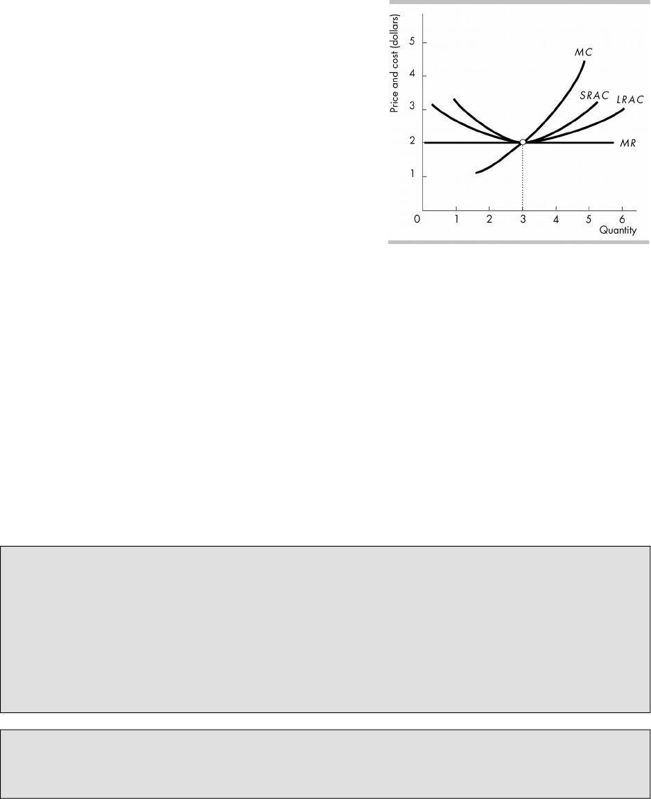
When the market supply curve shifts
rightward, the market price falls. Eventually
the price falls to equal the minimum ATC for
each rm in the industry and rms have
adjusted their plant size so they are
producing at the minimum long-run average
cost. At this price, rms in the industry no
longer make an economic prot and so rms
no longer enter the industry. The gure
illustrates this long-run equilibrium. In the
gure, LRAC is the long-run average cost
curve and SRAC is the short-run average
cost curve.
One di(erence between the old and new market equilibriums is that the number of
rms in the industry has risen and total quantity produced in the industry has
increased.
Exit
The e(ects of a decrease in market demand are the opposite of those outlined
above.
In the long run, competitive rms make zero economic prot (price = average total
cost) so that their owners make a normal prot.
Long Run Equilibrium
Long run equilibrium in a competitive market occurs when there is zero economic
prot and entry and exit have stopped.
Because markets are constantly experiencing new changes and shocks, it is rare to
see one in a state of long-run equilibrium, but each competitive markets reacts to
any new changes by pushing toward it.
Prot as a “signal”: When demand for a good increases so that the existing rms in an
industry make an economic prot, the economic prot indicates that consumers are willing
to pay a higher price for the good than they were willing to pay before the demand
increased. The economic prot for the rms is a signal from the consumers to the owners
of rms in other industries that society now values the availability of the good more highly
than the availability of goods from those other industries. These self-interested rm owners
choose to enter the industry in order to make an economic prot. Their self-interested
decisions promote the social interest by using more resources to produce those goods that
are more highly valued by society. The dynamic behavior of a perfectly competitive market
characterizes the “invisible hand” coined by Adam Smith.
Why would a rm stay in business if prot is zero? It is likely that you will hear this
question from at least one of your students. Remind them that the prot we’re measuring
is economic prot. Zero economic prot doesn’t necessarily mean that the rm isn’t
making any money. Rather, zero economic prot means that the prots the accountant is
© 2016 Pearson Education, Inc.
P E R F E C T C O M P E T I T I O N 1 2 3

reporting is exactly the same as the value of the rm’s best alternative. If the rm were to
move to its best alternative, it would make the same amount of prot. If a rm is making
zero economic prot, there isn’t any incentive to go anywhere else as there isn’t any place
that would generate a higher return for the rm. You may need to continue reminding your
students of this throughout this chapter.
An Economics in Action feature examines entry and exit using the personal computer
market and the farm equipment market.
V. Changes in Demand and Supply as Technology Advances
Change in Demand
Technological change can increase demand if it creates new applications for a
product or new products. Technological change can also decrease demand if new
ways of doing things or new products displace previous ones.
If demand increases, the price and economic prot rise. The economic prot
leads to entry, which increases market supply and causes the price to fall so that
eventually rms again make zero economic prot. The number of rms is greater
than before the increase in demand.
If demand decreases, the price falls and economic losses are created. Firms exit
the market, which raises the price and decreases the remaining rms’ economic
losses. Eventually the price rises so that the surviving rms make zero economic
prot. The number of rms is less than before the decrease in demand.
An Economics in the News case explores the e(ects of a decrease in demand for records
and taped music
Change in Supply
New, cost-saving technologies typically require new plant and equipment.
Consequently it takes time for new technology to spread throughout an industry.
Firms that adopt the new technology lower their costs and their supply curves shift
rightward. The price of the good falls but the rms with the new technology make an
economic prot.
Firms using the old technology incur economic losses. These rms either adopt the
new technology or else exit the industry. In the long run, all the rms use the new
technology and make zero economic prot.
Changes in technology brings only temporary economic prot to producers, but the
lower prices and better products that technological advances bring are permanent
gains for consumers.
An Economics in the News case explores the implications of technological changes that
have created falling costs to sequence DNA.
Do rms in perfectly competitive markets advertise? Firms in perfectly competitive
markets have no incentive to advertise because their product is indistinguishable from the
output of rival rms. Industry associations will sometimes advertize to increase demand for
the product as a whole. Brainstorming all the ads for agricultural products such as “Pork:
the other white meat,” and all the varieties of milk ads can be fun, but the point is that it
isn’t a pork producer or a dairy farmer creating the ad, but all of the pork producers or
dairy farmers paying dues to an industrial organization that then creates the ads.
Successful advertisements might lead to an economic prot in the short run, but in the
long run entry will force the rms back to zero economic prot.
© 2016 Pearson Education, Inc.
1 2 4 C H A P T E R 1 2
VI. Competition and E’ciency
Ecient Use of Resources
Resource allocation in a market is eAcient when society values no other use of the
resources more highly. Resource use is eAcient when production is such that the
marginal social benet of the good equals the marginal social cost of the good.
Choices, Equilibrium, and Eciency
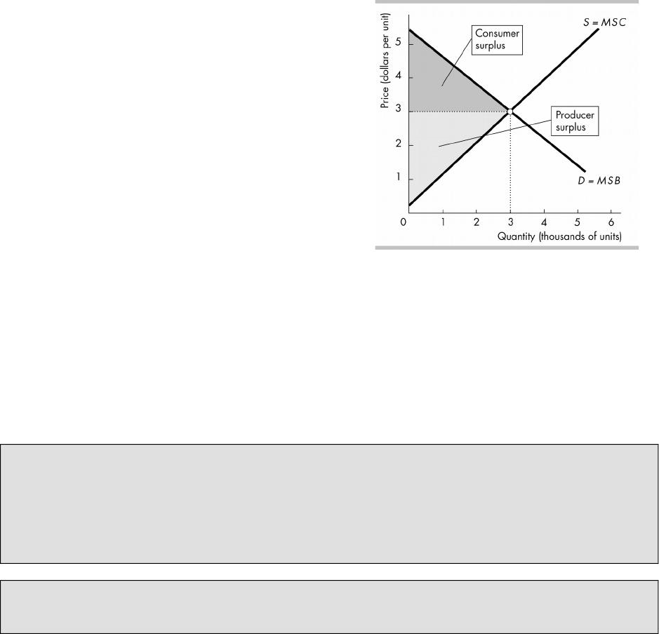
Consumers allocate their budgets to get
the most value out of them. Because
consumers get the most value out of their
budget, a consumer’s individual demand
curve for a good is the consumer’s
marginal benet curve for the good. If no
one else benets from the good other than
the consumers, then, as shown on the
gure, the market demand curve for a
good is the marginal social benet curve.
Firms maximize their prots in order to get
the most value out of their resources.
Firms make choices across all possible
allocations of their resources. A rm’s
supply curve for a good is its marginal
cost curve. If all the costs of production of
the good are paid by the producers, then, as shown in the gure, the market supply
curve for a good is the marginal social cost curve.
In a competitive equilibrium, the quantity demanded equals the quantity supplied. If
there are no externalities, the demand curve is the same as the marginal social
benet curve and the supply curve is the same as the marginal social cost curve, so
at the competitive equilibrium, the marginal social benet equals the marginal
social cost. Resource use is eAcient. Because resources are used eAciently, at the
competitive equilibrium there is no other allocation of resources that will generate
greater net benets to society. The gure shows this outcome, where resource use is
eAcient at the equilibrium quantity of 3,000 units.
Watching the work of the invisible hand: The power of the market to make rms
respond to consumers’ changing demands becomes visible to the student in this chapter.
When you teach the dynamics of rm entry and exit, do the analysis with a specic (and
current) example with which the students can identify. Have them pick an industry that has
grown and largely died in their lifetime (for me, VCRs, for them, DVDs at Blockbuster, or
video cameras or lm cameras). What has replaced it and how is society served by failure
as well as success?
Economics in the News analyzes the market for smart phone apps. It explains how the
rapid expansion of smartphones increased the demand for apps, thereby bring economic
prots to app producers.
© 2016 Pearson Education, Inc.
P E R F E C T C O M P E T I T I O N 1 2 5
Additional Problems
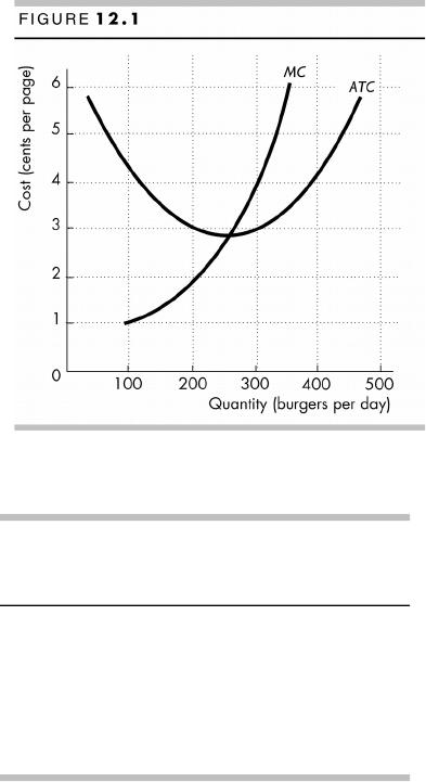
1. Bob’s is one of many burger stands along
the beach. Figure 12.1 shows Bob’s cost
curves.
a. If the market price of a burger is $4, what
is Bob’s prot-maximizing output?
b. Calculate the economic prot that Bob’s
makes.
c. With no change in demand or technology,
how will the price change in the long run?
2. Lucy’s Lasagna is a price taker that has
the costs shown in the table.
a. If lasagna sells for $7.50 a plate, what is
Lucy’s prot-maximizing output?
b. What is Lucy’s shutdown point?
c. Over what price range will Lucy leave the
lasagna industry?
d. Over what price range will other rms
with costs identical to Lucy’s enter the
industry?
e. What is the price of lasagna in the long run?
S o l u t i o n s t o A d d i t i o n a l P r o b l e m s
1. a. Bob’s prot-maximizing quantity is 300 burgers a day. Bob’s maximizes its prot by
producing the quantity at which marginal revenue equals marginal cost. In perfect
competition, marginal revenue equals price, which is $4 a burger. Marginal cost is $4
when 300 burgers a day are produced.
b. Bob’s economic prot is $300 a day. Prot equals total revenue minus total cost.
Total revenue equals $1,200 a day ($4 a burger multiplied by 300 burgers). The
average total cost of producing 300 burgers is $3.00 a burger, so total cost equals
$900 a day ($3.00 multiplied by 300 burgers). Prot equals $1,200 minus $900,
which is $300 a day.
c. The price will fall in the long run to $2.80 a burger. At a price of $4 a burger, rms
make economic prot. In the long run, the economic prot will encourage new rms
to enter the burger industry. As they do, the price will fall and economic prot will
decrease. Firms will enter until economic prot is zero, which occurs when the price
is $2.80 a burger (price equals minimum average total cost).
© 2016 Pearson Education, Inc.
Output
(plates per
hour)
Total cost
(dollars per
hour)
0 5
1 20
2 26
3 35
4 46
5 59
1 2 6 C H A P T E R 1 2
2. a. Lucy’s prot-maximizing output is 2 plates an hour. Lucy’s maximizes its prot by
producing the quantity at which marginal revenue equals marginal cost. In perfect
competition, marginal revenue equals price, which is $7.50 a plate. Marginal cost is
the change in total cost when output is increased by 1 plate an hour. The marginal
cost of increasing output from 1 to 2 plates an hour is $6 ($26 minus $20). The
marginal cost of increasing output from 2 to 3 plates an hour is $9 ($35 minus $26).
So the marginal cost of the second plate is half-way between $6 and $9, which is
$7.50. Marginal cost equals marginal revenue when Lucy produces 2 plates an hour.
b. Lucy’s shutdown point is at a price of $10 a plate. The shutdown point is the price
that equals minimum average variable cost. To calculate total variable cost, subtract
total xed cost ($5, which is total cost at zero output) from total cost. Average
variable cost equals total variable cost divided by the quantity produced. For
example, the average variable cost of producing 3 plates is $10 a plate. Average
variable cost is a minimum when marginal cost equals average variable cost. The
marginal cost of producing 3 plates is $10. So the shutdown point is a price of $10 a
plate.
c. Lucy will leave the industry if in the long run the price is less than $11 a plate. Lucy’s
Lasagna will leave the industry if it incurs an economic loss in the long run. To incur
an economic loss, the price will have to be below minimum average total cost.
Average total cost equals total cost divided by the quantity produced. For example,
the average total cost of producing 2 plates is $13 a plate. Average total cost is a
minimum when it equals marginal cost. The average total cost of producing 3 plates
is $11.67, and the average total cost of producing 4 plates is $11.50. Marginal cost
when Lucy’s produces 3 plates is $10 and marginal cost when Lucy’s produces 4
plates is $12. At 3 plates, marginal cost is less than average total cost; at 4 plates,
marginal cost exceeds average total cost. So minimum average total cost occurs
between 3 and 4 plates—$11 at 3.5 plates an hour.
d. Firms with costs identical to Lucy’s will enter at any price above $11 a plate. Firms
will enter an industry when rms currently in the industry are making economic
prot. Firms with costs identical to Lucy’s will make economic prot when the price
exceeds minimum average total cost, which is $11 a plate.
e. The price in the long run is $11 a plate. At $11 a plate, rms in the industry make
zero economic prot.
A d d i t i o n a l D i s c u s s i o n Q u e s t i o n s
1. Why do rms do what they do? Students should see how a clear
understanding of a perfectly competitive market justies rm behavior that
otherwise might appear somewhat peculiar:
Late night TV is full of zany TV commercials with rm owners who claim “I
must be crazy, because I’m losing money on every sale!” Why do they
advertise to increase sales if they’ll cause the owner to lose even more
money? At rst, it appears that these owners must be lying about “losing
money on every sale.” Yet their unlikely claim is potentially true, as the various
rms in their industry may currently face a market price above AVC, but below
ATC in the short run. In this case they would remain in business and continue
advertising, despite “losing money on every sale” because they are earning
revenues above their variable costs to at least help contribute toward paying
their xed cost obligations to their creditors.
Why do the same farmers always complain of losing money but never
seem to exit the industry? Point out that agriculture is a collection of highly
competitive markets where farming operations typically have an extremely
© 2016 Pearson Education, Inc.
P E R F E C T C O M P E T I T I O N 1 2 7
high capital-to-labor ratio. This fact makes the typical farm’s ratio of xed
costs to variable costs very high relative to most industries. Also, much of a
farmer’s capital is in the form farmland, which is diAcult to sell during falling
agriculture prices, lengthening the farmer’s short run time frame. In this case,
the dollar di(erence between market price and minimum AVC will be rather
large. As long as market price exceeds AVC, the farmer will minimize losses by
continuing to produce output over an extended short run time frame.
2. What is implied about e$ciency if the average cost of producing a
good exceeds the price people are willing to pay for it? Remind the
students that a rm’s cost curves reOect the opportunity cost to society of the
rm using the resources to make the goods in its market (the resources could
be making goods in some other market that could bring benets to society).
The demand curve reOects the value society places on each quantity of goods
produced. If the price people are willing to pay is determined by the market
supply and demand and the going market price is less than the opportunity
cost of producing the last unit of the good, using more resources to increase
output creates fewer net benets for society than could be generated if the
resources were used elsewhere in other markets.
What happens to the resources that were used by a rm for
production when that rm exits the industry? Point out that when price
falls below ATC, this generates an economic loss for the rm. This is a signal
from a society of consumers to the owner of the resources that he or she will
benet from reallocating the resources to making di(erent goods and services
from the same resources. Society also stands to benet from this switch.
How can an increase in net benets to society be generated from the
systematic destruction of rms leaving the market? A famous economist
named Joseph Schumpeter coined the phrase “creative destruction” to
describe the dynamics of a competitive market. While the productive capacity
of a perfectly competitive industry facing declining consumer demand is
ultimately destroyed, the resources themselves are not destroyed. They are
simply released to rms in other markets to create goods and services that are
relatively more valuable to society. This “destruction” of an industry creates
goods of greater social value in another industry. That is Schumpeter’s
“creative destruction.”
3. What makes all the self-interested rms adopt the latest available
technology for producing at the lowest opportunity cost possible over
time? Emphasize that competitive rms cannot increase their economic
prots by raising their price, so they must search for ways to increase
economic prot through lowering production costs. This means that rms are
constantly seeking out the latest production technologies to nd a cost
advantage over their competitors. If the other rms failed to adopt this
low-cost production technology, they would su(er an economic loss when
those that do adopt the technology lower their prices to increase market share.
Firms that refuse to adopt the technology must then match a lower market
price to retain their market shares, causing them to bear an economic loss and
face an eventual exit from the market.
4. Discuss whether there are economies of scale or diseconomies of
scale in class size at colleges and universities. Does it matter if the
“output” is measured in tuition dollars and costs or in student
success as measured by grades? Does technology impact the answer?
This situation can be fun to explore. Can a great teacher supported by
excellent technology be best used in a huge lecture class? Are there some
© 2016 Pearson Education, Inc.
1 2 8 C H A P T E R 1 2
types of instruction, like experimental labs, where increasing class size might
lead to disaster? Why do colleges advertise their average class size and do
parents and students care? How might the educational “plant” and equipment
di(er to support various choices in class size?
5. Using the global corn market, consider the impact of increasing
demand for ethanol made from corn in the short and long run. The
increase in demand for ethanol raises the price of corn and thereby increases
corn farmers’ economic prot…at least in the short run. But in the long run,
the economic prot leads existing farmers to plant more corn and more corn
farmers to enter the. These long-run changes increase the supply of corn,
thereby lowering the price of corn and decreasing corn farmers’ economic
prot. Entry (and expansion) continues until, in the long run, corn farmers’
economic prot equals zero. At that point entry ceases and the corn market is
back in long-run equilibrium.
© 2016 Pearson Education, Inc.
P E R F E C T C O M P E T I T I O N 1 2 9