
W H AT I S E C O N O M I C S ? 1 3 1
T h e B i g P i c t u r e
Where we have been:
Chapter 12 relies heavily on the productivity and cost analysis material of
Chapter 11, the marginal analysis and e$ciency issues introduced in Chapter
2 and Chapter 5, and the concept of economic pro&t introduced in Chapter 10.
Where we are going:
Chapter 12 is the &rst of four chapters that explore the price and output
decisions of &rms under various market characteristics. Chapter 12 studies
perfect competition, Chapter 13 studies monopoly, Chapter 14 studies
monopolistic competition, and Chapter 15 studies oligopoly. All four chapters
use cost curves, marginal analysis, and the concept of e$ciency.
N e w i n t h e Tw e l f t h E d i t i o n
Some material is presented in a more streamlined manner that increases clarity
for students. The chapter continues to explore the impact technology has on
changing the market, both on the demand and supply sides. A new Worked
Problem section has been added. The Worked Problem provides a market demand
schedule and a &rm’s average and marginal cost schedules. It then shows the
students how to calculate the &rm’s shutdown point and, assuming there are
1,000 identical &rms, how to &nd the market equilibrium price and quantity. It
uses these results to show the students how to determine if &rms will enter or exit
the market and what will be the long-run equilibrium. To include the new Worked
Problem without lengthening the chapter, some problems have been removed
from the Study Plan Problem and Applications. These problems are in the
MyEconLab and are called Extra Problems.
12PERFECT
COMPETITION
C h a p t e r
131

L e c t u r e N o t e s
Perfect Competition
Firms in perfect competition face the maximum amount of competition because
there are many competing &rms, each of which produces an identical product.
Firms in perfect competition maximize their pro&t by producing where MR = MC.
Perfect competition leads to an e$cient allocation of resources.
I. What is Perfect Competition?
Perfect competition is an industry in which
Many &rms sell identical products to many buyers
There are no restrictions on entry into the industry
Established &rms have no advantage over existing ones
Sellers and buyers are well informed about prices
How Perfect Competition Arises
These characteristics of perfect competition arise when the minimum e$cient scale
for a &rm is small relative to the size of the entire market. The minimum e$cient
scale is the smallest output at which long-run average costs are minimized.
What markets satisfy the characteristics of perfect competition? Have the
students consider the markets for goods with which they are familiar to see if any meet the
strict criteria for perfect competition. The markets that come closest are agricultural
markets, though others such as lawn service, plumbing, gas stations, and so on, also come
close. Students sometimes “worry” that these markets are not exact examples of perfect
competition. Reassure them that the model of perfect competition gives us a great deal of
understanding into the workings of extremely competitive real world markets and the real
world &rms in the markets.
If there aren’t really any perfectly competitive markets, what use is studying
perfect competition? The perfect competition model serves as a benchmark and its
predictions work in a wide range of real markets. Set the scene for appreciating the power
of the perfect competition model with a physical analogy. Explain that physicists often use
the model of a “perfect vacuum” to understand our physical world. For example, to predict
how long it will take a 50 pound steel ball to hit the ground if it is dropped from the top of
the Empire State Building, you will be very close to the actual time if you assume a perfect
vacuum and use the formula that applies in that case. Friction from the atmosphere is
obviously not zero, but assuming it to be zero is not very misleading. In contrast, if you
want to predict how long it will take a feather to make the same trip, you need a much
fancier model! Economists use the model of perfect competition in a similar way to
understand our economic world. Emphasize to students that, although no real world
industry meets the full de&nition of perfect competition, the behavior of &rms in many real
world industries and the resulting dynamics of their market prices and quantities can be
predicted to a high degree of accuracy by using the model of perfect competition.
Price Takers
Firms in perfect competition are price takers, meaning that a &rm that cannot
in<uence the market price and so it sets its own price equal to the market price.
What is a price taker? Spend a few minutes providing intuition to ensure that your
students understand why &rms in perfect competition are “price takers.” On the one hand,
they could o=er to sell for a lower price, but they’d be giving pro&ts away because they can
sell all they want at the going market price. On the other hand, they can ask for a higher
price but not even one consumer will pay because consumers know where to buy an exact
substitute at a lower price.
Economic Prot and Revenue
Firms operating in perfect competition seek to maximize economic pro&t, which is
the di=erence between total revenue (the price of the &rm’s output multiplied by
the quantity sold) and its total opportunity cost of production
Because the &rm is a price taker, its marginal revenue—which is the change in
total revenue that results in a one-unit increase in the quantity sold—is equal to the
market price and remains constant as output sold increases.
The &rm’s demand is perfectly elastic and the &rm’s demand curve is a horizontal
line at the market price.
II. The Firm’s Output Decision
Marginal Analysis and the Supply Decision
The &rm produces the quantity of output for which the di=erence between total
revenue and total cost is at its maximum because this di=erence is its economic
pro&t.
Marginal analysis can be used to determine the pro&t maximizing quantity. The &rm
compares the marginal revenue (which remains constant with output) to the
marginal cost (which changes with output) of producing di=erent levels of output.
When MR > MC, then the extra revenue from selling one more unit exceeds the
extra cost of producing one more unit, so
the &rm increases its output to increase
its pro&t.
When MR < MC, then the extra cost of
producing one more unit exceeds the
extra revenue from selling one more unit,
so the &rm decreases its output to
increase its pro&ts
When MR = MC, then the extra cost of
producing one more unit equals the extra
revenue from selling one more unit, so
the &rm’s pro&t is maximized at this level
of output.
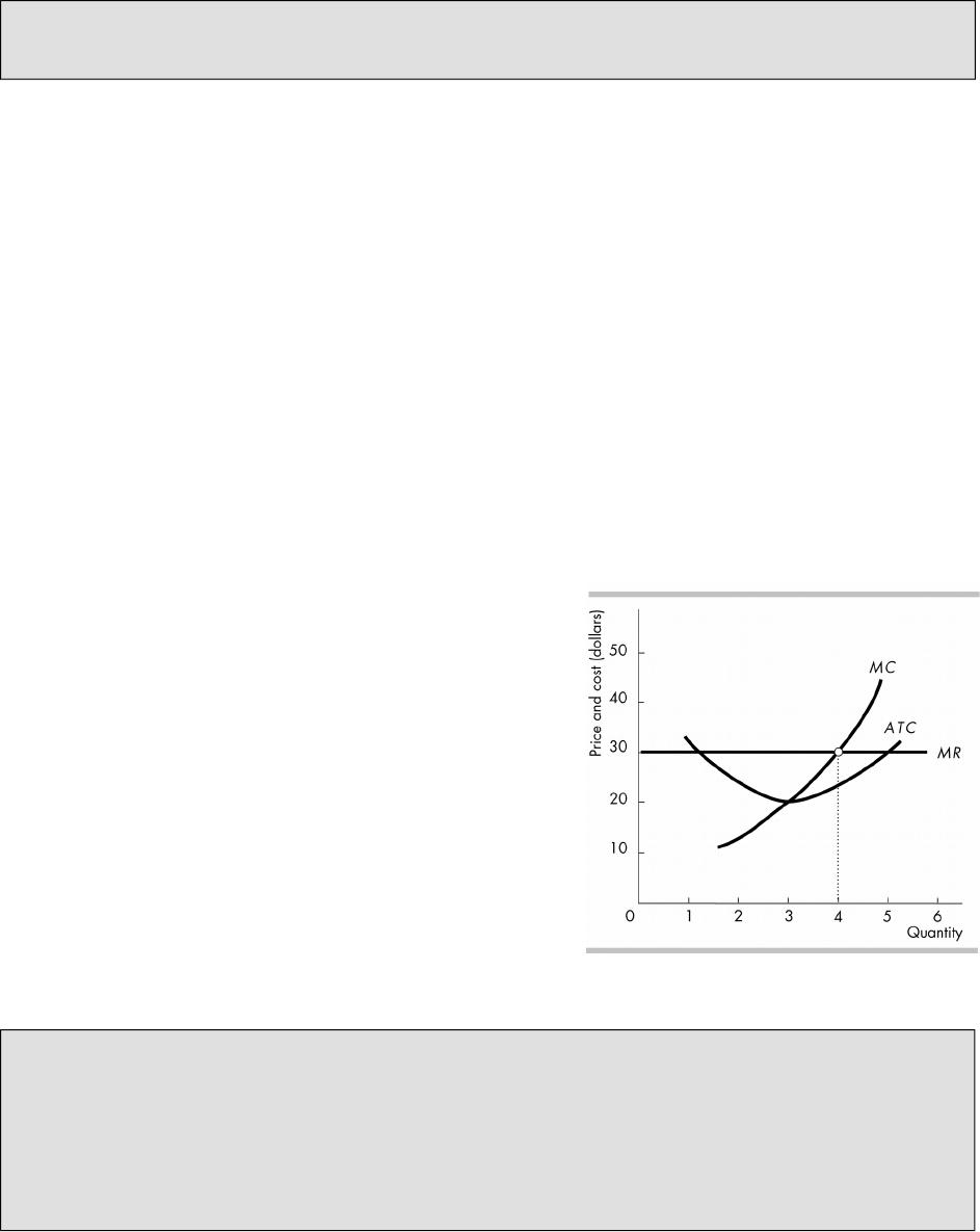
In the &gure the &rm produces 4 units of
output because that is the quantity that
sets the &rm’s marginal cost equal to its marginal revenue, that is, MR = MC. The
&rm then charges the going market price of $30 for its good.
What’s the point? Students &nd the topic of competitive market dynamics challenging.
Part of their problem is that understanding the dynamics requires a strong understanding
of the cost curves of the previous chapter, yet many of them still have only a shaky grasp
of that important material. So emphasize the cumulative nature of economics and remind
the students of the huge payo= from mastering material a bite at a time.
You also can help your students by emphasizing the two primary goals of this chapter: (1)
To derive the market supply curve in a competitive industry and (2) to deepen your
students’ understanding of how competition among self-interested consumers and
producers will move society’s resources from less valued uses to more highly valued uses,
achieving an e$cient allocation in the eyes of society.
Temporary Shutdown Decision
The &rm will temporarily shut down in the short run when price falls below the
shutdown point, which is the output and price that just allows the &rm to cover its
total variable cost. The minimum AVC is the lowest price at which the &rm will
operate because if it operated with a lower price, the &rm’s loss would be greater
than if it shut down. (The loss when the &rm shuts down is equal to its &xed cost.)
The &rm will continue operating in the short run even if it incurs an economic loss as
long as the price exceeds the minimum AVC.
Why would a restaurant open on days it knows business will be bad? Monday is
typically the slowest day in the restaurant industry. So why do so many restaurants stay
open on Monday? The answer is that even if a restaurant incurs an economic loss on
Monday, it still might increase its total pro&t by remaining open. The point is that as long
as the restaurant can cover all its variable costs—the cost of the food, the cost of the
servers, and so on—it likely will be able to pay some of its &xed costs using the revenue left
over after paying its variable costs. As long as the restaurant can pay some of its &xed
costs on Monday, its total pro&t by staying open exceeds what its total pro&t would be if it
closed. So losing money on Monday might be good business!
Students often have a hard time understanding why operating at an economic loss can be
the best action for a &rm owner. The key is emphasizing:
The &rm’s short-run decisions are made after some irreversible commitments have
generated sunk costs.
The &rm considers only avoidable future costs when making decisions. Unavoidable
costs have no impact on the decision (other than to learn from them).
For the &rm to continue to produce output, the &rm needs only to receive revenues
that exceed any avoidable costs, not necessarily all total costs.
Basically, the goal of pro&t maximization does not guarantee that the &rm will earn a
positive economic pro&t in the short run. Sometimes the best the &rm can do is to minimize
its economic loss.
The Firm’s Supply Curve
As long as the &rm remains open, it produces
where MR = MC. So the &rm’s supply curve is
its MC curve above the minimum AVC. At
prices below the minimum AVC, the &rm
shuts down and supplies zero.
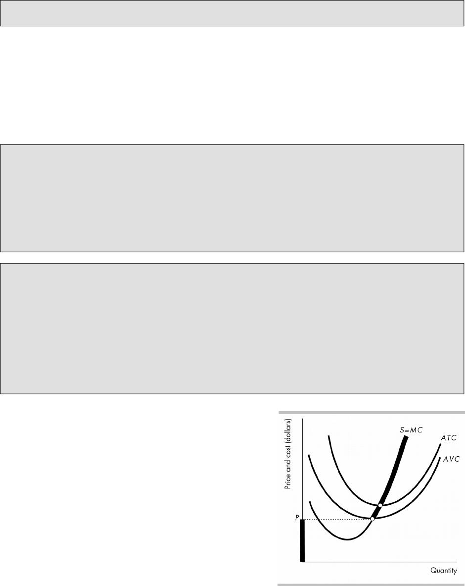
The &gure shows the &rm’s supply curve as
the heavy dark line.
At prices less than the minimum average
variable cost, which equals P in the
&gure, the &rm shuts down and supplies
zero.
At prices greater than the minimum
average variable cost, the &rm supplies
along its marginal cost curve. Hence the
&rm’s marginal cost curve is its supply, indicated in the &gure by the S = MC
curve.
III. Output, Price, and Pro-t in the Short Run
The short run is a situation in which the number of &rms is &xed. In the short run, market
demand and market supply interact to determine the price and quantity produced in a
perfectly competitive market.
Market Supply in the Short Run
The short-run market supply curve shows the quantity supplied by all the &rms
in the market at each price when each &rm’s plant and number of &rms remain the
same. The quantity supplied in the industry at any price is the summation of all
quantities supplied by each &rm at that price, so the short-run industry supply curve
is the horizontal summation of all the &rms’ supply curves.
Short-run Equilibrium
Market demand and short-run market supply determine the market price and
market output. Each &rm takes the market price as given, and produces its pro&t
maximizing output.
A Change in Demand
Changes in market demand in<uence the output and the entry or exit decisions
made by &rms.
An increase in market demand shifts the market demand curve rightward and raises
the market price. Each &rm responds by increasing its quantity supplied.
A decrease in market demand shifts the market demand curve leftward and
decreases the market price. Each &rm responds by decreasing its quantity supplied.
Prots and Losses in the Short Run
In the short run, even though &rms attempt
to maximize pro&t, they may end up
breaking even or incurring an economic loss.
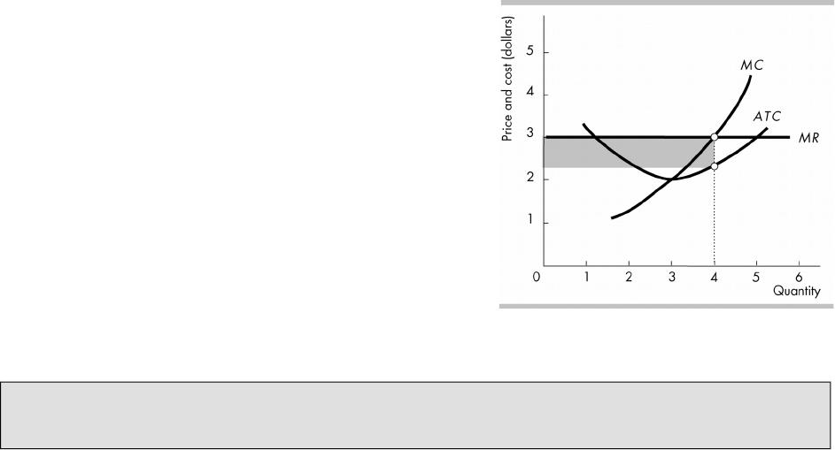
The total economic pro&t (or loss) is equal to
(P − ATC) × q.
If the price exceeds the ATC, the &rm
makes an economic pro&t (as illustrated
in the &gure).
If the price equals the ATC, the &rm
“breaks even” by making zero economic
pro&t. In this case, the entrepreneur
makes a normal pro&t.
If the price is less than the ATC, the &rm
incurs an economic loss.
An Economics in Action application considers the situation of Harley Davidson after a
decrease in the market demand. Harley Davidson cut production and laid o= workers. One
plant was temporarily idled and other jobs were lost permanently.