W H AT I S E C O N O M I C S ? 1 7 7
A n s w e r s t o t h e R e v i e w Q u i z z e s
Page 248
1. Distinguish between the short run and the long run.
The short run is a period of time during which the quantity of at least one factor of
2. Why is a sunk cost irrelevant to a &rm’s current decisions?
Sunk cost is irrelevant because it cannot be changed by any decision. It is already
Page 252
1. Explain how the marginal product and average product of labor change as
the labor employed increases (a) initially and (b) eventually.
Initially, as the quantity of labor is increases, the &rm experiences increasing
marginal returns, which means that the marginal product increases as more labor
is employed. Increasing marginal returns occur because hiring additional workers
allows the workers to specialize and become more productive. Eventually, the &rm
will experience diminishing marginal returns which means that the marginal
product decreases as more labor is employed. Decreasing marginal returns occur
2. What is the law of diminishing returns? Why does marginal product eventually
diminish?
The law of diminishing returns states that as a &rm uses more of a variable factor
of production with a given quantity of &xed factors of production, the marginal
3. Explain the relationship between marginal product and average product.
1
1
OUTPUT AND
COSTS
177
1 7 8
As the quantity of labor initially increases the &rm experiences increasing marginal
returns and the marginal product of labor increases. The marginal product of labor
is greater than the average product over this range of labor, so the average
Page 259
1. What relationships do a &rm’s short-run cost curves show?
The marginal cost (MC), average total cost (ATC) and average variable cost (AVC)
curves are all related in the short run:
When the MC curve lies above (lies below) the AVC curve, the AVC curve rises
(falls) with output. This implies that as output increases, the MC curve cuts
2. How does marginal cost change as output increases (a) initially and (b)
eventually?
At small outputs, marginal cost decreases as output increases because of greater
3. What does the law of diminishing returns imply for the shape of the marginal
cost curve?
The law of diminishing returns states: As a &rm uses more of a variable factor of
production, with a given quantity of the &xed factor of production, the marginal
4. What is the shape of the AFC curve and why does it have this shape?
Average &xed cost (AFC) equals total &xed cost divided by total product. As the
5. What are the shapes of the AVC curve and the ATC curve and why do they
have these shapes?
The average variable cost (AVC), and average total cost (ATC) curves are both
U-shaped.
The marginal cost (MC) curve shows how total cost changes when output
ATC is the sum of average &xed cost (AFC) and AVC. Initially the ATC curve falls
178
W H A T I S E C O N O M I C S ? 1 7 9
Page 263
1. What does a &rm’s production function show and how is it related to a total
product curve?
A &rm’s production function is the relationship between the maximum output
2. Does the law of diminishing returns apply to capital as well as labor? Explain
why or why not.
The law of diminishing returns applies to capital as well as labor. The marginal
product of capital is the change in the total product resulting from a one-unit
3. What does a &rm’s LRAC curve show? How is it related to the &rm’s short-run
ATC curves?
The long-run average cost curve (LRAC) shows the relationship between the lowest
attainable ATC and output when both plant size and labor are varied. The LRAC
curve re9ects the minimum possible ATC the &rm can attain for any given level of
4. What are economies of scale and diseconomies of scale? How do they arise?
What do they imply for the shape of the LRAC curve?
Economies of scale are features of a &rm’s technology that lead to falling long-run
average cost (LRAC) as output increases. As plant size increases, the minimum
attainable average total cost (ATC) for each plant size falls with output.
5. What is a &rm’s minimum e;cient scale?
Minimum ecient scale is the smallest quantity of output at which long-run
A nsw e r s t o t h e S t ud y P l a n Pr ob l e ms a nd
A p p l i c a t i o n s
179
180
1. Which of the following news items involves a short-run decision and which
involves a long-run decision? Explain.
January 31, 2008: Starbucks will open 75 more stores abroad than originally
predicted, for a total of 975.
February 25, 2008: For three hours on Tuesday, Starbucks will shut down every
single one of its 7,100 stores so that baristas can receive a refresher course.
This decision is a short-run decision. It involves increasing the quality of Starbucks’
June 2, 2008: Starbucks replaces baristas with vending machines.
This decision is a short-run decision. It involves changing two of Starbucks’ factors
July 18, 2008: Starbucks is closing 616 stores by the end of March.
This decision is a long-run decision. It decreases the quantity of all of Starbucks’
Use the table to work Problems 2 to 6.
The table sets out Sue’s Surfboards’ total product
schedule.
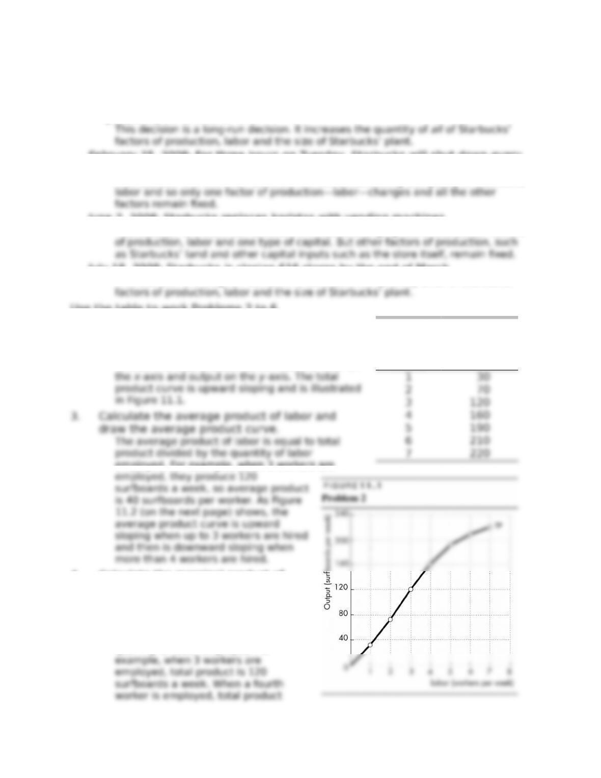
2. Draw the total product curve.
To draw the total product curve measure labor on
employed. For example, when 3 workers are
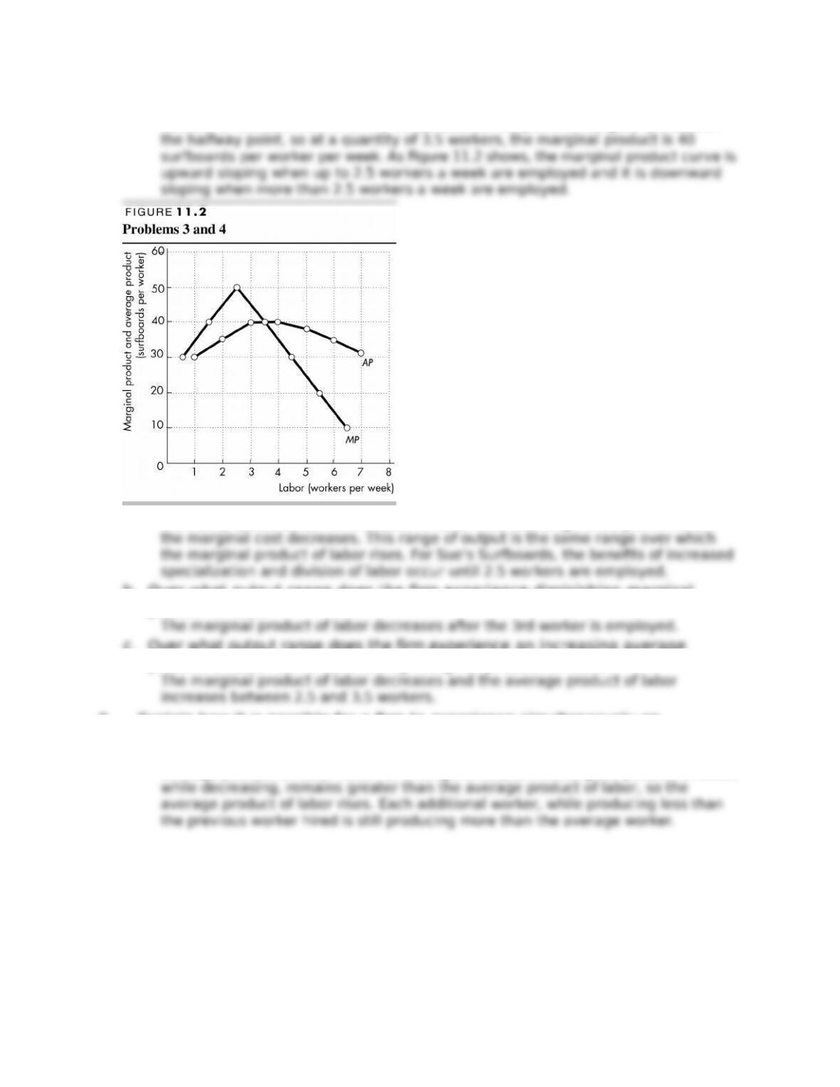
4. Calculate the marginal product of
labor and draw the marginal product
curve.
The marginal product of labor is equal
to the increase in total product that
results from a one-unit increase in the
quantity of labor employed. For
Labor
(workers
per
week)
Output
(surfboards
per week)
180
W H A T I S E C O N O M I C S ? 1 8 1
increases to 160 surfboards a week. The marginal product of increasing the
number of workers from 3 to 4 is 40 surfboards. We plot the marginal product at
5. a. Over what output range does
Sue’s Surfboards enjoy the bene&ts of
increased specialization and division of
labor?
The &rm enjoys the bene&ts of
increased specialization and division of labor over the range of output for which
b. Over what output range does the &rm experience diminishing marginal
product of labor?
c. Over what output range does the &rm experience an increasing average
product of labor but a diminishing marginal product of labor?
6. Explain how it is possible for a &rm to experience simultaneously an
increasing average product but a diminishing marginal product.
As long as the marginal product of labor exceeds the average product of labor, the
average product of labor rises. For a range of output the marginal product of labor,
181
182
Use the following data to work Problems 7
to 11.
Sue’s Surfboards, in Problem 2, hires
workers at $500 a week and its total &xed
cost is $1,000 a week.
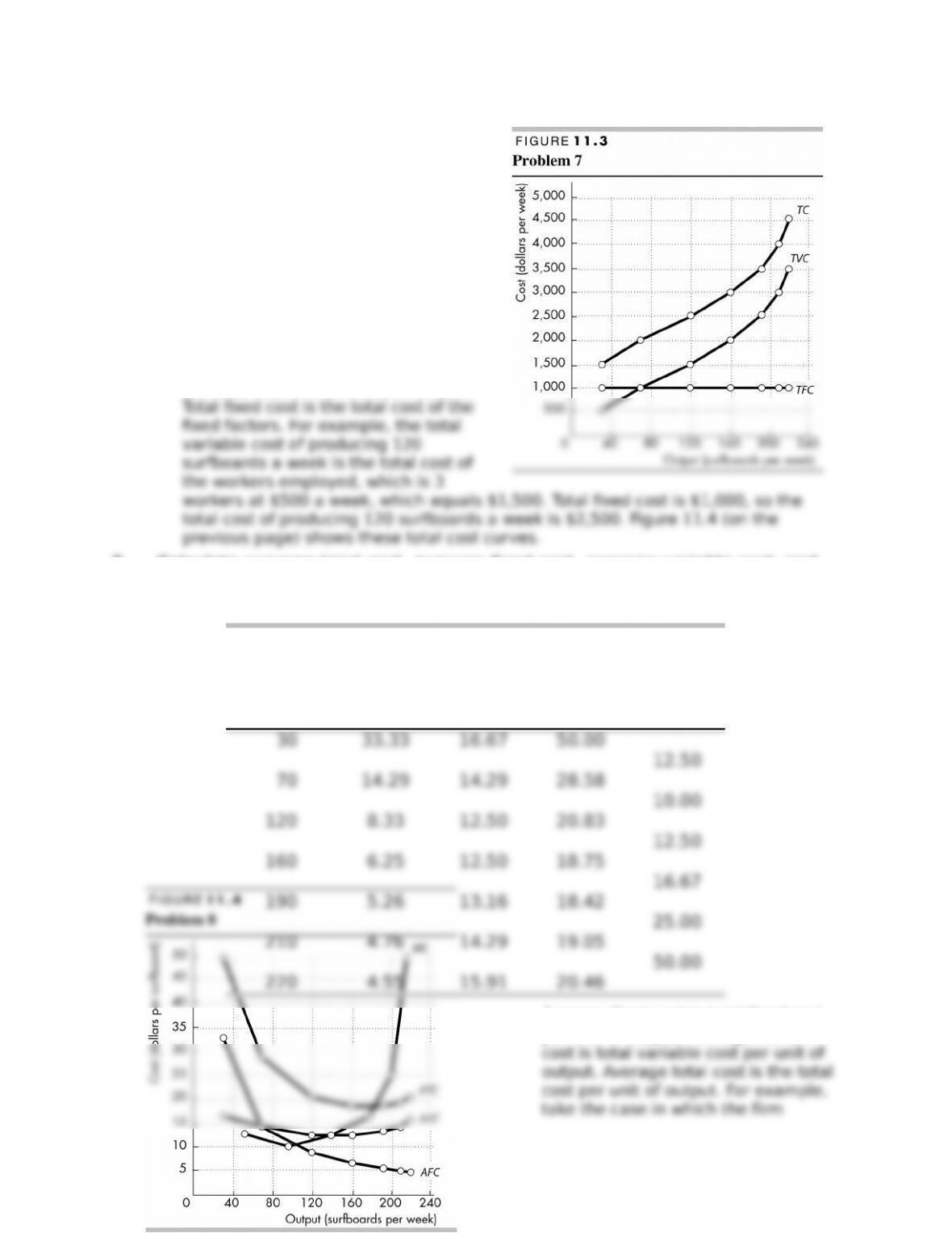
7. Calculate total cost, total variable
cost, and total &xed cost of each
output in the table. Plot these points
and sketch the short-run total cost
curves passing through them.
Total cost is the sum of the costs of all
the factors of production that Sue’s
Surfboards uses. Total variable cost is
the total cost of the variable factors.
8. Calculate average total cost, average &xed cost, average variable cost, and
marginal cost of each output in the table. Plot these points and sketch the
short-run average and marginal cost curves passing through them.
Output
(surfboard
s)
AFC
(dollars
per
surfboar
d)
AVC
(dollars
per
surfboar
d)
ATC
(dollars
per
surfboar
d)
MC
(dollars
per
surfboar
d)
Average &xed cost is total &xed cost
per unit of output. Average variable
182
W H A T I S E C O N O M I C S ? 183
makes 160 surfboards a week. Total &xed cost is $1,000, so average &xed cost is
$6.25 per surfboard; total variable cost is $2,000, so average variable cost is
$12.50 per surfboard; and, total cost is $3,000, so average total cost is $18.75 per
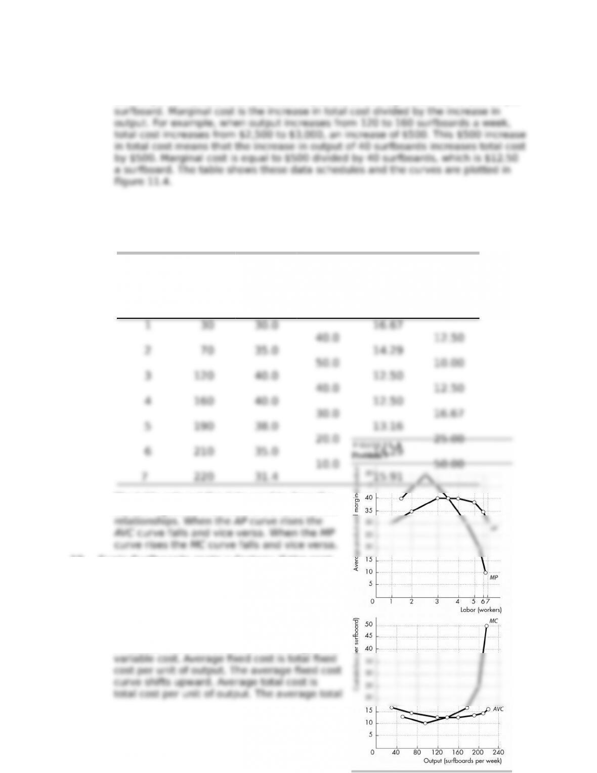
9. Illustrate the connection between Sue’s AP, MP, AVC, and MC curves in graphs like those
in Fig. 11.7.
Labor
(worker
s)
Output
(surfboar
ds)
AP
(surfboar
ds per
worker)
MP
(surfboar
ds per
worker)
AVC
(dollars
per
surfboar
d)
MC
(dollars
per
surfboar
d)
The table sets out the data used to draw the
curves. Figure 11.5 shows the curves and the
10. Sue’s Surfboards rents a factory. If the rent
rises by $200 a week and other things
remain the same, how do Sue’s Surfboards’
short-run average cost curves and marginal
cost curve change?
The rent is a &xed cost, so total &xed cost
increases. The increase in total &xed cost
increases total cost but does not change total
183
1 8 4
11. Workers at Sue’s Surfboards negotiate a wage increase of $100 a week per
worker. If other things remain the same, explain how Sue’s Surfboards’
short-run average cost curves and marginal cost curve change.
The increase in the wage rate is a variable cost, so total variable cost increases.
The increase in total variable cost increases total cost but total &xed cost does not
184
Use the following data to
work Problems 12 to 14.
Jackie’s Canoe Rides rents
canoes at $100 per day
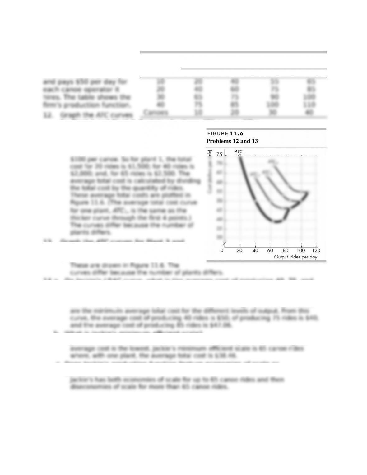
12. Graph the ATC curves
for Plant 1 and Plant 2. Explain why these ATC curves diIer.
To &nd the average total cost for each
plant, at the diIerent levels of output add
the cost of the workers, $50 per worker,
and the &xed cost, the cost of the canoes,
14.a. On Jackie’s LRAC curve, what is the average cost of producing 40, 75, and
85 rides a week?
The long-run average total cost curve is illustrated in Figure 11.6 as the thicker
curve. It is comprised of the parts of the short-run average total cost curves that
b. What is Jackie’s minimum e;cient scale?
Jackie’s minimum e;cient scale is the smallest quantity at which the long-run
c. Does Jackie’s production function feature economies of scale or
diseconomies of scale?
Labor
(workers
per day)
Output
(rides per day)
Plant 1 Plant 2 Plant 3 Plant 4